Longitudinal Experiments
Longitudinal Experiments. Larry V. Hedges Northwestern University Prepared for the IES Summer Research Training Institute July 28, 2010. What Are Longitudinal Experiments?. Longitudinal experiments are experiments with repeated measurements of an outcome on the same people Examples


Longitudinal Experiments
E N D
Presentation Transcript
Longitudinal Experiments Larry V. Hedges Northwestern University Prepared for the IES Summer Research Training Institute July 28, 2010
What Are Longitudinal Experiments? Longitudinal experiments are experiments with repeated measurements of an outcome on the same people Examples Experiments with immediate and delayed posttests Experiments that track individuals over many performance periods (e.g., school years) Experiments that intend to impact growth rate Experiments that make repeated measurements of behavior (e.g., teacher behavior) to increase precision of measurement
Why Do Longitudinal Experiments? Three reasons for doing longitudinal experiments • More than one discrete endpoint is of interest (e.g., immediate vs delayed outcome) • Several measures of the outcome are necessary to increase precision or reduce variation (e.g., teacher behavior is averaged over many occasions) • The time course of treatment effect (growth trajectory) is of interest (e. g., an intervention is intended to increase the rate of vocabulary acquisition in preschool children) In all three cases, linear combinations of outcomes may be of interest
Why Do Longitudinal Experiments? Unless different outcomes are being compared, there is no need to use longitudinal methods! But, if different outcomes are being compared, outcomes are not independent Thus, longitudinal methods must be used
Modeling Longitudinal Experiments We can describe models for longitudinal experiments via ANOVA or HLM notation We can analyze longitudinal experiments via either ANOVA or HLM There are big advantages to using HLM notation for these models There are even bigger advantages to using HLM for analyses of these models Hence we will primarily use HLM notation in our discussion of longitudinal experiments
Discrete Endpoints The design will typically have at least three levels Measures are nested (clustered) within individuals, individuals are nested (clustered) within schools Level 1 (measures within individuals) Level 2 (individuals within schools) Level 3 (schools) Let Yijk, the observation on the kth measure for the jth person in the ith school
Discrete Endpoints, Schools Assigned(No Covariates) Level 1 (measure level) Yijk = β0ij + εijk ε ~ N(0, σW2) Level 2 (individual level) β0ij = γ00i + η0ijη ~ N(0, σI2) Level 3 (school level) γ00i = π00 + π01Ti + ξ0i ξ ~ N(0, σS2) Where we code the (centered) treatment Tj = ½ or - ½ , so that π01is the ANOVA treatment effect
Discrete Endpoints(Unconditional Model) Note that the εijk’s are not just measurement errors but also contain differences between outcomes for each individual Similarly the η0ij‘s are between individual differences in these quantities Then the ξ0i‘s are between-school differences on these quantities That makes the unconditional model difficult to interpret
Discrete Endpoints, Schools Assigned(Comparing Early and Delayed Outcome) Level 1 (measure level) Yijk = β0ij + β1ijDijk + εijk ε ~ N(0, σW2) Level 2 (individual level) β0ij = γ00i + η0ij η~ N(0, ΣI) β1ij = γ10i + η1ij Level 3 (school level) γ00i = π00 + π01Ti + ξ0i ξ~ N(0, ΣS) γ10i = π10 + π11Ti + ξ1i Note that the η0ij’s and η1ij’s can be correlated as can the ξ0i’s and ξ1i’s
Discrete Endpoints, Individuals Assigned(Comparing Early and Delayed Outcome) Level 1 (measure level) Yijk = β0ij + β1ijDijk + εijk ε ~ N(0, σW2) Level 2 (individual level) β0ij = γ00i + γ01iTi + η0ij η~ N(0, ΣI) β1ij = γ10i + γ11iTi + η1ij Level 3 (school level) γ00i = π000 + ξ00i γ01i = π010 + ξ01iξ~ N(0, ΣS) γ10i = π100 + ξ10i γ11i = π110 + ξ11i Note that the η0ij’s and η1ij’s can be correlated as can the ξ’‘s and ξ’s
Discrete Endpoints(Comparing Early and Delayed Outcome) Note that, in this model, the εijk’s can be interpreted as measurement errors Similarly the η0ij‘s are between individual differences in these quantities and the intraclass correlation ρI = σI2/(σs2 + σI2 + σW2) is a true (individual level) reliability coefficient Then the ξ0i‘s are between-school differences on these quantities and the intraclass correlation ρS = σS2/(σs2 + σI2 + σW2) is a true (school level) reliability coefficient
Discrete Endpoints, Schools Assigned(Comparing Early and Delayed Outcome) Covariates can be added at any level of the design But remember that covariates must be variables that cannot have been impacted by treatment assignment Thus time varying covariates (at level 1) are particularly suspect since they may be measured after treatment assignment
Average of Several Measures The design will typically have at least three levels Measures are nested (clustered) within individuals, individuals are nested (clustered) within schools Level 1 (measures within individuals) Level 2 (individuals within schools) Level 3 (schools) Let Yijk, the observation on the kth measure for the jth person in the ith school with p measures per individual
Average of Several Measures(Treatment Assigned at the School Level) Level 1 (measure level) Yijk = β0ij + εijk ε ~ N(0, σW2) Level 2 (individual level) β0ij = γ00i + η0ijη ~ N(0, σI2) Level 3 (school level) γ0i = π00 + π01Ti + ξ0i ξ ~ N(0, σS2) Where we code the (centered) treatment Tj = ½ or - ½ , so that π01is the treatment effect
Average of Several Measures(Treatment Assigned at the Individual Level) Level 1 (measure level) Yijk = β0ij + εijk ε ~ N(0, σW2) Level 2 (individual level) β0ij = γ00i + γ01iTij + η0ijη ~ N(0, σI2) Level 3 (school level) γ00i = π00 + ξ0i ξ~ N(0, ΣS) γ01i = π01 + ξ1i Where we code the (centered) treatment Tj = ½ or - ½ , so that π01is the treatment effect
Average of Several Measures Note that, in this model, the εijk’s can be interpreted as like (item level) measurement errors Then the β0ij‘s can be interpreted as individual level measures (for the jth person in the ith school) Thus the η0ij‘s are between individual differences in these quantities and the quantity ρI = σI2/(σs2 + σI2 + σW2/p) is a true (individual level) reliability coefficient Then the ξ0i‘s are between-school differences on these quantities and the quantity ρS = σS2/(σs2 + σI2 + σW2/p) is a true (school level) reliability coefficient
Growth Trajectories The problem of fitting growth trajectories is more complicated It requires choosing a form for the growth trajectories It also requires choosing a form for the model of individual differences in these growth trajectories Many forms are possible, but polynomials are conventional for two reasons: • Any smooth function is approximately a polynomial (Taylor’s Theorem) • Polynomials are simple
What is a Polynomial Model? Yijk = β0ij + β1ijtijk + β2ijtijk2 + β3ijtijk3 + εijk Typically, tijk is a measure of time at the measurement for the jth person in the ith school at the tth measurement We typically center the measurements at some point for convenience (often the middle of the time span) Centering strategy determines the interpretation of the coefficients of the growth model Note that the measurements do not have to be at exactly the same time for each person
Understanding a Polynomial Model Yijk = β0ij + β1ijtijk + β2ijtijk2 + β3ijtijk3 + εijk How do we interpret the coefficients? β0ij is the intercept at the centering point β1ij is the linear rate of growth at the centering point β2ij is the acceleration (rate of change of linear growth) at the centering point β3ij is the rate of change of the acceleration (often negative leading to flattening out of growth curves at the extremes)
Understanding a Polynomial Model Consider the quadratic growth model to understand acceleration with mean centering Thus you can see that the linear growth rate at time t is In other words, the linear growth rate increases with t andthe only place where the linear growth rate isβ1ijis the middle
Understanding a Polynomial Model Thus β1ij is the linear rate of growth at the centered value (here, the middle) If β2ij > 0, the linear growth rate will be larger above the centered value and smaller below the centered value Centering at other values than the middle can make sense if that is where growth trajectory is of interest and if the model fits the data For example, centering at the end gives coefficients with interpretable rates at the end of the growth period
Understanding a Polynomial Model Consider the quadratic growth model to understand acceleration with mean centering Thus you can see that the acceleration at time t is In other words, the acceleration increases with t and the only place where the acceleration isβ2ijis the middle
Understanding a Polynomial Model Thus β2ij is the acceleration of growth at the centered value (here the middle) If β3ij > 0, the acceleration will be larger above the centered value and smaller below the centered value Centering at other values than the middle can make sense if that is where growth trajectory is of interest and if the model fits the data For example, centering at the end gives coefficients with interpretable rates at the end of the growth period
Linear Growth (Centered)β0 = 5, β1 = 1, β2 = 0.00, β3 = 0.00
Quadratic Growth (Centered)β0 = 5, β1 = 1, β2 = 0.05, β3 = 0.00
Cubic Growth (Centered)β0 = 5, β1 = 1, β2 = 0.05, β3 = -0.01
Linear, Quadratic, and Cubic Growth (Centered)β0 = 5, β1 = 1, β2 = 0.05, β3 = -0.01,
Selecting Growth Models Several considerations are relevant in selecting a growth model First is how many repeated measures there are: The maximum degree is one less than the number of measures (linear needs 2, quadratic needs 3, etc.) However the estimates of growth parameters are much better if there are a few additional degrees of freedom But the most important consideration is whether the model fits the data! Unfortunately, this is not always completely unambiguous
Selecting Growth Models Individual growth trajectories are usually poorly estimated HLM models estimate average growth trajectories (via average parameters) and variation around that average: These are much more stable Estimates of individual growth curves can be greatly improved by using empirical Bayes methods to borrow strength from the average This may make sense if there all the individuals in the groups are sampled from a common population It can be problematic if some individuals are dramatically different
Selecting Analysis Models One issue is selecting the growth model to characterize growth A different, but related, issue is selecting how treatment should impact growth Should it impact linear growth term? Should it impact the acceleration? Which impact is primary? How does looking at multiple impacts weaken the design? What if impacts are in opposite directions?
Longitudinal Experiments Assigning Treatment to Schools In the language of experimental design, adding repeated measures adds another factor to the design: A measures factor The measures factor is crossed with individuals, treatments, and clusters Schools are nested within the treatment factor and individuals are nested within school by treatments Repeated measures analysis of variance can be used to analyze these designs, but we will not pursue that point of view Instead we will use the HLM notation
Longitudinal Experiments Assigning Treatment To Schools Level 1 (measures) Yijk = β0ij + β1ijtijk + β2ijtijk2 + εijk Level 2 (individuals) β0ij = γ00j + η0ijη~ N(0, ΣI) β1ij = γ10j + η1ij β2ij = γ20j + η2ij Level 3 (schools) γ00j = π00 + π01Ti + ξ0j ξ~ N(0, ΣS) γ01j = π10 + π11Ti + ξ1j γ20j = π20 + π21Ti + ξ2j
Longitudinal Experiments Assigning Treatment To Schools This model has three trend coefficients in each growth trajectory Note that there are 3 random effects at the second and third level This means that 6 variances and covariances must be estimated at each level This may require more information to do accurately than is available at the school level It is often prudent to fix some of these effects because they cannot all be estimated accurately
Longitudinal Experiments Assigning Treatment Within Schools In the language of experimental design, adding repeated measures adds another factor to the design: A measures factor The measures factor is crossed with individuals, treatments, and clusters The treatment factor is crossed with schools and individuals are nested within school by treatments Repeated measures analysis of variance can be used to analyze these designs, but we will not pursue that point of view
Longitudinal Experiments Assigning Treatment Within Schools Level 1 (measures level) Yijk = β0ij + β1ijt + β2ijt2 + εijk ε ~ N(0, σW2) Level 2 (individual level) β0ij = γ00j + γ01jTj + η0ijη~ N(0, ΣC) β1ij = γ10j + γ11jTj + η1ij β2ij = γ20j + γ21jTj + η2ij Level 3 (school level) γ00j = π00 + ξ00j ξa0~ N(0, ΣS) γ01j = π10 + ξ01j ξa1~ N(0, ΣTxS) γ10j = π00 + ξ10j γ11j = π00 + ξ11j γ20j = π00 + ξ20j γ21j = π00 + ξ21j
Longitudinal Experiments Assigning Treatment Within Schools This model has three trend coefficients in each growth trajectory Note that there are 6 random effects at the third level This means that 15 variances and covariances must be estimated at the third level This requires a great deal of information to do accurately It is often prudent to fix some of these effects because they cannot all be estimated accurately However there is some art in this, and sensitivity analysis is a good precaution
Longitudinal Experiments Covariates can be added at any level of the design But remember that covariates must be variables that cannot have been impacted by treatment assignment Thus time varying covariates (at level 1) are particularly suspect since they may be measured after treatment assignment
Power Analysis Power computations for longitudinal experiments are doable, but depend on parameters that may not be well known For example reliability of trend coefficients When parameters such as these are known, the computations are straightforward, but there is relatively little information about them that can be used for planning To make matters worse, the values of some parameters (such as reliability) depend on the number of measures Thus it is often necessary to rely on values of variance components
Power Analysis Still some generalizations are possible • Power increases with the number of measures • Power increases with the length of time over which measures are made (except for β0ij) • Power increases with the precision of each individual measure These factors impact different trend coefficients differently Clustering increases the complexity of computations
Power Analysis Pilot data (or data from related studies, perhaps non-experimental ones) is more important in planning longitudinal experiments Longitudinal experiments to look at growth trajectories are attractive, but this is an area at the frontier of practical experience Research is ongoing to produce better methods for power analysis of longitudinal experiments that will be practically useful