Download
1 / 28
280 likes | 400 Vues
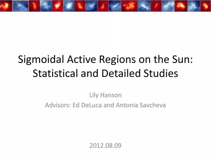
Sigmoidal Active Regions on the Sun: Statistical and Detailed Studies. Lily Hanson Advisors: Ed DeLuca and Antonia Savcheva 2012.08.09. Overview. Introduction to sigmoids What they are What makes them interesting Our catalog Model of NOAA region 11474 (sigmoid S66)

E N D
Sigmoidal Active Regions on the Sun: Statistical and Detailed Studies Lily Hanson Advisors: Ed DeLuca and Antonia Savcheva 2012.08.09
Overview • Introduction to sigmoids • What they are • What makes them interesting • Our catalog • Model of NOAA region 11474 (sigmoid S66) • Model creation and selection • Properties of the modeled region • Current sheets and QSL maps
Introduction to Sigmoids • Solar Active Region (AR) with forward or backward S-shape in soft x-rays. (Orientation is somewhat correlated to hemisphere.) • Long-lasting sigmoid lifetime: days or weeks • Transient sigmoid lifetime: hours • May be near a coronal hole, other active region(s), or sunspots. S64 XRT image S55 XRT image S56 XRT image
S52a, S52b AIA 335Å S56 XRT image S65, S66 AIA 335Å S46, S47, S48 XRT image
Relevance of Sigmoids • Shown to be a good predictor for flares and coronal mass ejections (CMEs).[Canfield et al. 1999, 2007] • First step to understanding general behavior is to gather as much information as possible: this is the value of creating a catalog.
The Sigmoid Catalog • Full catalog ranges from Feb 2007 – May 2012 and contains 66 sigmoidal ARs, found by inspecting XRT synoptic images. • Sigmoids are subjectively rated based on the clarity of their S-shape. We focused on the higher-rated sigmoids. • Priority was given to regions for which we have high-resolution data from AIA. • Catalog is most complete for sigmoids during Aug 2010 – May 2012. (15 sigmoids)
Data Collected for the Catalog • Spreadsheet with the following information: • Sigmoid ID (which we assigned) • Rating of sigmoid clarity • NOAA region number • AR start/end date/time • Position on solar disk • Size (arcsec) of longest axis • Aspect ratio (long axis / short axis) • S-shape start/end date/time • Date/time of strongest S-shape • Orientation (straight or inverted) • Hemisphere where sigmoid occurs • EUV or Hα filament visible • Sunspots associated with AR • Coronal hole(s) nearby • Other AR(s) nearby • GOES flares (date/time and class) • Flare-associated phenomena: filament eruptions, flare ribbons, transient coronal holes, post-flare loops • Videos of each AR in 335Å and 171Å (full disk and zoomed-in) • High-cadence videos of each GOES flare in 335Å, 304Å, and 171Å (zoomed-in only) • Daily screenshots of filaments (Hα) and sunspots (4500Å) from SolarMonitor.org (full disk only) • Screenshot of “Best S” time for each sigmoid in XRT and in AIA 335Å (full disk only) • Plots of positive and negative magnetic flux changing with time, created from magnetogram data
The Sigmoid Catalog Number observed Number observed Number observed Number observed
The Sigmoid Catalog The catalog lets us combine data: flare events, S-shape, disk center crossing, and flux can be plotted together against time.Some flux plots show a parabolic trend, which may require geometric corrections. Number observed Flux ×1021 [Mx] Green shading represents S-shape. Time [hours] Flux ×1021 [Mx] Solid vertical line shows when center of solar disk is crossed.Dashed vertical lines represent flare events. Time [hours]
The Sigmoid Catalog • Flare phenomena (relatively rare using GOES classification): • Filament eruptions (failed or successful) • Flare ribbons • Transient coronal holes • Post-flare loops
The Sigmoid Catalog • Flare phenomena S39, C4.4 flare: successful filament eruption, flare ribbons, and post-flare loops AIA 171Å S46, C6.7 flare: failed filament eruption AIA 171Å
The Sigmoid Catalog • Flare phenomena S66, flare not GOES classified:flare ribbons AIA 304Å S66, flare not GOES classified:transient coronal holes AIA 335Å
Model of S66 / AR 11474 • 2012 May 3 – 14 (11.7 days) • S-shape visible from May 4 – 11 (6.8 days) • Filament seen in EUV and Hα • Small sunspot present for part of lifetime • Modeled at 05:38 on 2012 May 08, shortly before eruption at 09:26 (shown in videos from the previous slide).
Creating a Model with CMS2 • Line-of-sight (LoS) magnetogram data is used to calculate the potential field of the entire sun. Assumptions: • The magnetic field at the photosphere is radial and is specified by the magnetograms. • All magnetic field lines at the outer surface of the computational volume are radial.
Creating a Model with CMS2 • A flux rope is inserted into the calculated potential field along the filament path, connecting positive and negative flux elements. The rope’s poloidal and axial flux values are different for each model. High resolution magnetogram contours superimposed on AIA 304Å image
Best Fit Model • After a relaxation process, the best model’s field lines lie closest to the observed coronal loops (red). Best fit: Model 8. Model 1 Axial Flux [Mx] Model 8 High resolution magnetogram contours on XRT image
Basic Properties of Model 8 • Poloidal flux: -1 × 10¹⁰Mx cm-1 • Axial flux: 7 × 10²⁰ Mx • Fit parameter: 0.0064 Rsun(from comparison with five coronal loops) • Potential energy: 1.06 × 1032 ergs • Free energy: 2.96 × 1031 ergs • Relative helicity: -2.41 × 1042 Mx2
Current Structures in Model 8 • A cross-sectional plot of the modeled currents shows a unique topology with four zones. Field lines in each zone create the S-shape. z-axis Yellow line becomes s-axis y-axis y-axis s-axis z-axis x-axis x-axis s-axis
Further Studyof the Model 60k iterations z-axis • Cross-sectional currents at 30k and 60k iterations show the flux rope is rising. We ran the model for another 80k iterations to mimic the region’s time evolution. s-axis 80k iterations z-axis s-axis 120k iterations z-axis s-axis 140k iterations z-axis s-axis
Conclusions • We have created a catalog of strong sigmoids from Aug 2010 – May 2012. • This lets us identify variations and unifying characteristics. • Analyzing typical behavior and evolution will improve space weather forecasting capabilities. • S66 is modeled by a flux rope on the filament, with poloidal and axial flux given by model 8. • Unique topological features are apparent in current cross-section. • Slight instability of model can be used to imitate and study changes with time.
Future Work • The slightly unstable model of S66 will be used to compare topological structures (QSLs) with observations of energetic particle precipitation (flare ribbons) to investigate the magnetic field configuration around reconnection sites.
References and Bibliography • “Field Topology Analysis of a Long-Lasting Coronal Sigmoid”, A. Savcheva, A. van Ballegooijen, E. DeLuca, 2012, ApJ, 744, 78 • “Nonlinear Force-Free Modeling of a Long-Lasting Coronal Sigmoid”, A. Savcheva and A. van Ballegooijen, 2009, ApJ, 703, 1766 • “YOHKOH SXT Full-Resolution Observations of Sigmoids: Structure, Formation, and Eruption”, R. Canfield et al., 2007, ApJ, 671, L81 • “Sigmoidal Morphology and Eruptive Solar Activity”, R. Canfield et al., 1999, GRL, Vol 26, No 6, 627
Acknowledgements and Special Thanks • Dr. Edward DeLuca and Antonia Savcheva for their extensive knowledge and valuable help • Dr. Adriaan van Ballegooijen for assistance with CMS2 • CfA researchers and support staff for organizing the REU programs, answering questions, and welcoming us to the CfA • NSF Grant ATM-0851866 for making it all possible • CfA grad students, postdocs, and other well-wishers for exquisite baked goods and bloodthirsty games of Mafia • The Solar and Astro REU crews for teaming up to find ice cream, the beach, and creative solutions to the Two Refrigerator Problem • Boston for its many Wonders and Marvels
Thank you! … Questions? AIA 335Å
Formation of Sigmoids • Long-lasting sigmoids are theorized to form from shearing in a potential arcade. Generally we assume that a twisted flux rope is present, which is held in place by the overlying arcade. Cartoon showing formation of a flux rope in the presence of shearing,from A.A. van Ballegooijen and P.C.H. Martens, "Formation and eruption of solar prominences," ApJ 343, 971 (1989) Copied from Hudson’s Solar Cartoon Archive.
Relaxation of Flux Rope Models • Non-Linear Force-Free Fields (NLFFF) • Models are relaxed by magnetofrictional relaxation with hyperdiffusion for 60k iterations. • The models’ fit quality is inspected at 30k iterations.
Comparison of Selected Models Coronal Loops(selected from XRT image) Model 1Poloidal flux: -5e9Axial flux: 1e20 Model 18Poloidal flux: -5e10Axial flux: 1e21 Model 8Poloidal flux: -1e10Axial flux: 7e20 High-resolution magnetogram contours superimposed on XRT image High-resolution magnetogram contours with model field lines
QSL Maps and Flare Ribbons • A Quasi-Separatrix Layer (QSL) marks the boundary between regions of strong magnetic field divergence. These are possible sites for reconnection and energy release. • Flare ribbons are a sign of energy release that may be occurring at a QSL. We can compare QSL maps at different heights to flare ribbon shape. QSL Map superimposed on AIA 304 Å image with flare ribbons.