Algorithms for Discovering Patterns in Sequences
Algorithms for Discovering Patterns in Sequences. Raj Bhatnagar University of Cincinnati. Outline. Applications of Sequence Mining Genomic Sequences Engineering/Scientific Data Analysis Market Basket Analysis Algorithm Goals Temporal Patterns Interesting Frequent Subsequences

Algorithms for Discovering Patterns in Sequences
E N D
Presentation Transcript
Algorithms for Discovering Patterns in Sequences Raj Bhatnagar University of Cincinnati
Outline • Applications of Sequence Mining • Genomic Sequences • Engineering/Scientific Data Analysis • Market Basket Analysis • Algorithm Goals • Temporal Patterns • Interesting Frequent Subsequences • Interesting Frequent Substrings (with mutations) • Detection of Outlier sequences
Why Mine a Dataset? Discover Patterns: • Associations • A subsequence pattern follows another • Help make a prediction • Clusters • Typical modes of operation • Temporal Dependencies • Events related in time • Spatial Dependencies • Events related in space
Example Problems From various domains • Engineering • Scientific • Genomic • Business
Multivariate Time Series • Multivariate time series data is a series of multiple attributes observed over a period of time at equal intervals • Examples: stocks, weather, utility, sales, scientific, sensor monitoring and bioinformatics
Spatio-Temporal Patterns Goal: Find patterns in space-time dimensions for phenomena Issues: Simultaneous handling of space and time dimensions Problem: How to handle large complexity of algorithms Phenomena in space-time
Discover Interesting Subsequences AAAAAAAAGGGGGGG-(10,15)-CTGATTCCAATACAG actgatAAAAAAAAGGGGGGGggcgtacacattagCTGATTCCAATACAGacgt aaAAAAAAAAGGGGGGGaaacttttccgaataCTGATTCCAATACAGgatcagt atgacttAAAAAAAAGGGGGGGtgctctcccgattttcCTGATTCCAATACAGc aggAAAAAAAAGGGGGGGagccctaacggacttaatCCTGATTCCAATACAGta ggaggAAAAAAAAGGGGGGGagccctaacggacttaatCCTGATTCCAATACAG Blue pattern sequence may have upto k substitutions
Main Sequence Mining Tasks • Finding frequent patterns • Doing similarity search • Clustering of time series • Periodicity detection • Finding temporal associations • Summarization • Prediction
31 0 1 2 3 4 5 6 7 8 9 10 11 12 13 14 15 16 17 18 19 20 21 22 23 24 25 26 27 28 29 30 32 33 34 35 36 37 38 39 Finding Frequent Substrings • Two Main Approaches: • Generalized Suffix Trees (Linear Time) • Find Least Common Substrings (Linear Time) abacebc . abcdobd . abaaebd . eoaoobd . abceoad . • GST generated considering the substrings starting at location #0 of each string is: (0) < root > - (8) ab - (10) c – (11)dobd - (15) 8 - (35) e0ad – (39) 32 - (18) a – (19) aebd – (23) 16 - (3) cebc – (7) 0 - (24) e0a00bd - (31) 24
Finding Frequent Substrings • Recursively generate the GST with each string truncated by removing the first character Original strings: abacebc . abcdobd . abaaebd . eoaoobd . abceoad . Truncated strings: bacebc . bcdobd . baaebd . oaoobd .bceoad . (0) < root > - (8) b - (10) dobd - (14) 8 - (31) e0ad – (35) 29 - (16) a – (17) aebd – (21) 15 - (3) cebd – (7) 1 - (22) 0a00bd - (28) 24
Results after Phase-I • Substrings generated after Phase-I are:
Phase2: Subsequence Hypotheses Result of Phase 1: string size(s) profiles(G) size(G) ABa---- 3 {0,2} 2 AB----- 2 {0,1,2} 3 --a---- 1 {0,2,3} 3 ----*bd 3 {1,3} 2 -----bd 2 {1,2,3} 3 Result after Phase 2: subsequence size(T) profiles(R) size(R) AB---bd 4 {1,2} 2 --a--bd 3 {2,3} 2
Merging Profile Sets • Two sets of profiles are similar and will be merged together if: Size(Intersection(P1, P2)) ≥ threshold Size(Union(P1, P2 )) where P1 and P2 any two sets and threshold is user-defined
Generalizing Substring Patterns • Core subsequences can be written in the form of regular expressionor regex • Each symbol is considered replaceable by preceding or following alphabet E.g. for the substring, aba – eb - - regex will be [ab]{1}[abc]{1}[ab]{1}.{1}[def]{1}[abc]{1}.{2}
Generalization of Sequence Patterns • Hypothesis T specifies a core subsequenceshared by the set of profiles R • Core subsequences and set R, affected by various factors such as loss of information • T is considered as seedof hypothesis
What is Achieved • Discover: • Partial-sequence temporal hypotheses • identities of profiles for each temporal hypothesis
Histone Cluster Fourier Results ORF Process Function Peak Phase Order Cluster Order YBL002W chromatin structure histone H2B S 424 789 YBL003C chromatin structure histone H2A S 441 790 YBR009C chromatin structure histone H4 S 417 791 YBR010W chromatin structure histone H3 S 420 795 YDR224C chromatin structure histone H2B S 432 794 YDR225W chromatin structure histone H2A S 437 796 YNL030W chromatin structure histone H4 S 418 792 YNL031C chromatin structure histone H3 S 430 793 YPL127C chromatin structure histone H1 S 448 788 ------------------------------------------------------------------------------------------- YBL002W CC ab dccaCBBBabc*BCCCA* xcCBCbbcccACACCBBbaabbb* dcABCaaabbBCxBBBa cccbABCBBBBBab YBL003C CC ab cdcbBCBBbacaBCCC** cbCCCAbcccaCCCCBA*bcbbaA bcABBb*ab*AxABBAa cb*baBBCBBBB*b YBR009C xC *x ddcaCCBBaab*BCCB*a xcCCBbccccbCBCBBa*bbxaAB baB*AaA*bxdBaBBBB cccbABCCCBABAb YBR010W BC aA ccc*CBBAbbc*BCCBAa bbCCB*ccdbbCBCCCAAxbcaAB bbA*Ab*bbAAxaBBB* bccbaBBBBB*Bab YDR224C BC aa ccc*CCB*abbaBBCA*b cbCCB*cccbbCCCCCAAcccaAB caBAAaabbAAxaBBBA cccb*BBCBBBBAb YDR225W CC *b cdcaCCC*abbbBCCBAa cbCCC*bccbaCCCBCBAbccbaB cbAA*a*bbAAxaBBBB bccbaBCBBBBB*b YNL030W CC bb dccACCBAabb*CBCBAa cbCCBacccbbCCCCB*AbbcaAB b*AaAbabbBxBaA*BA cccb*BCCBBBB*b YNL031C CC ab cccABCB*abb*BCCAAa bbCCB*bccbbBBCBC*Abbbb*B bAAAAbabbBAxaA*B* bcbb*BBCBAA**b YPL127C Da bb dcaBBCBAabb*BBBBAa cbBCABbcdbaBABBCBBbcbaAB ccBBBB*bcbABBxAAb bccbABBCBBBA*a ^.{4}[cdx]{2}.{3}[BCx]{1}.{3}[abx]{1}.{3}[BCDx].{7}[BCx]{1}.{3}[bcdx]{2}.{5}[BCx]{1}.{33}[BCx]{1}[ABCx]{1}.{5}$ CC-b--c---------BCC-----C---bcc----C-------b----A-----b-----------b-B--B----b YBL002W CCabdccaCBBBabc*BCCCA*xcCBCbbcccACACCBBbaabbb*dcABCaaabbBCxBBBacccbABCBBBBBab YBL003C CCabcdcbBCBBbacaBCCC**cbCCCAbcccaCCCCBA*bcbbaAbcABBb*ab*AxABBAacb*baBBCBBBB*b YDR225W CC*bcdcaCCC*abbbBCCBAacbCCC*bccbaCCCBCBAbccbaBcbAA*a*bbAAxaBBBBbccbaBCBBBBB*b YNL031C CCabcccABCB*abb*BCCAAabbCCB*bccbbBBCBC*Abbbb*BbAAAAbabbBAxaA*B*bcbb*BBCBAA**b ++x----x+++x---x+++xxx--+++x----x+x+++xx-x--xxxxx+x-x--x++x+x+x--x-x++++++xx- 5,6,10,14,18,26,30,31,37,71,72 String-Based Results Regular Expression Generalization
Example 2 with Yeast Cell Data Original Hypothesis ORF Process Function Peak Phase Order Cluster Order YBR009C chromatin structure histone H4 S 417 791 YBR010W chromatin structure histone H3 S 420 795 YDR224C chromatin structure histone H2B S 432 794 YDR225W chromatin structure histone H2A S 437 796 YLR300W cell wall biogenesis "exo-beta-1,3-glucanase" G1 381 756 YNL030W chromatin structure histone H4 S 418 792 YNL031C chromatin structure histone H3 S 430 793 Not classified as cell cycle related: YBR106W, YBR118W, YBR189W, YBR206W, YCLX11W, YDL014W, YDL213C, YDR037W, YDR134C, YGL148W, YKL009W, YLR449W, YNL110C, YPR163C ^.{46}[bcx]{1}.{1}[ABx]{1}[aA*x]{1}[AB*]{1}[abx]{1}[aA*x]{1}.{1}[abcx]{1}[ABx]{1}.{1} [ABCx]{1}[ab*x]{1}[ABx]{1}.{1}[ABCx]{1}.{15}$ New Genes Included After Localized Generalization New Regular Expression
Algorithms for LCS • Substring : continuous sequence of characters in a string • Subsequence : obtained by deleting zero or more symbols in a given string abcdefghia Substrings : cdefg, efgh, abcd Subsequences: ade , cefhi, abc, aia
Longest Common Subsequence • LCS is common subsequence of maximal length between two strings String 1 : abcdabcefghijk String 2: xbcaghaehijk LCS = bcaehijk, Length of LCS = 8
Finding LCS • Brute Force has exponential time complexity in the length of string • Dynamic Programming can find LCS in O(mn) time and space complexity • Length of LCS can be found in O(min(m,n)) space complexity and O(mn) time complexity
Main Sequence Mining Tasks • Finding frequent patterns • Doing similarity search • Clustering of time series • Periodicity detection • Finding temporal associations • Summarization • Prediction
Finding the LCS Length Recursive Formulation: LCS[i, j] = 0, if i = 0 or j = 0 LCS[i-1, j-1] + 1, if i, j > 0 and ai = bj max(LCS[i, j-1], LCS[i-1, j]), if i, j > 0 and ai ≠ bj
Findingthe LCS Length Recursive Formulation: LCS[i, j] = 0, if i = 0 or j = 0 LCS[i-1, j-1] + 1, if i, j > 0 and ai = bj max(LCS[i, j-1], LCS[i-1, j]), if i, j > 0 and ai ≠ bj Iterative solution is more efficient than recursive
Finding the LCS Length: Algorithm lcs_length(A, B) { // A is a string with length m // b is another string with length n , m>=n // L is an array to keep intermediate values in Dynamic Programming for (i = m; i >= 0; i--) for (j = n; j >= 0; j--) { if (A[i] = '$' || B[j] = '$') L[i,j] = 0; //end of strings else if (A[i] == B[j]) L[i,j] = 1 + L[i+1, j+1]; else L[i,j] = max(L[i+1, j], L[i, j+1]); } return L[0,0]; }
Sequential Clustering • Clustering is partitioning the data in equivalence classes • Data is input one or few times • Unique classification based on input order • Simple and fast for large data
Main Sequence Mining Tasks • Finding frequent patterns • Doing similarity search • Clustering of time series • Periodicity detection • Biological Sequence Problems
Multivariate Time Series • Multivariate time series data is a series of multiple attributes observed over a period of time at equal intervals • Examples: stocks, weather, utility, sales, scientific, sensor monitoring and bioinformatics
Time Series Analysis Tasks • Finding frequent patterns • Doing similarity search • Clustering of time series • Periodicity detection • Finding temporal associations • Prediction
Why temporal association rules? • More information about correlations between frequent patterns • Contains richer information than knowledge frequent patterns • Helps to build diagnostic and prediction tools
Finding temporal associations: recent work • Mannilla - Discovery of frequent episodes in event sequences [2], 1997 • Das - Rule Discovery from Time Series [1], 1998 • Kam - Discovering temporal patterns for interval-based events [3], 2000 • Roddick - Discovering Richer Temporal Association Rules from Interval-based Data [4], 2004 • Mörchen - Discovering Temporal Knowledge in Multivariate Time Series [5], 2004
Research Issues • Finding richer set of temporal relationships { contains, follows, overlaps, meets, equals …} than sequence mining does {follows} • Robustness of rules - room for noise in patterns • Understanding temporal relationships at different levels of abstraction • Efficient algorithms to find patterns with noise and temporal associations.
Temporal Association Rules Frameworks • Kam[1] uses Allens temporal relations to find rules • Roddick[4] uses state sequence framework similar to Höppner [6] • Mörchen [5] is based onUnification-based Temporal Grammar.
Allen’s relationships Above figure is presented from [1]
Problem Given a multivariate time series, minimum support for number of occurrences, minimum pattern length find all the temporal association rules (similar to A1) less than size k
dimensionalityreduction, discretization and symbolic representation Frequent pattern enumeration aaaeffdaaaaaaaaacccaaaaaaaaaaedefggcbabaacfgfc… dccbbccdccdeedcdcdeecccdddeeecdeccccddegedbcdc… dddcbbcfffeeegffcbcdeeefffffecbbaaaaaacffecbbb… clustering multivariate time series sequences Temporal association rule discovery Summarization and visualization {aaaaaaaa, bbbaaa, bbaaa, eeef, aaac, eaaa ...} {cdee, dccde, deed, ddeeec, eeec, ccccc,edddd …} {fff,fffe,aaaaa,fecbb,ddcb,bbbbc,bbbbc,cbbb…} {aaaaaaaa} {bbba,bba,..} {eeef…} {aaac,eaaa …}… {cdee}{dccde…}{deed,ddeeec,eeec…}{ccccc…}{edddd…}… {fff,fffe…}{fecbb…}{ddcb…}{bbbbc,bbbbc,cbbb…} … frequent patterns clusters 1.{aaaa,aaac,aaae,abaa…}followed by{cbb,ccbb,cccbb…} 2.{bbbbb,cbbbbbc,…}followed by{baaaa,aaaaaaa,aaaaaa …} overlaps {aaaa,aaac,aaae…} 3.{dccccdd,ccccdd} contains{aaaaa,aaaa } 4. … 5. … …. Temporal rules Summarized rule
Mining in 3 steps • Find all frequent patterns in each dimension along with all the occurrence. • Cluster the similar Patterns to form equivalence classes • Find temporal associations between these equivalence classes using iterative algorithm
Step 1: Finding Frequent Patterns • The Data in each dimension is quantized to form a string ( equal frequency, equal interval, SAX, persist etc…) [8]. • Enhanced Suffix Tree is constructed for this string using O(n) Algorithm [7]. • All the Frequent patterns along with the locations are enumerated in Linear Time by complete traversal of Tree.