Download
1 / 12
120 likes | 261 Vues
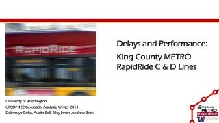
Delays and Performance: King County METRO RapidRide C & D Lines. University of Washington URBDP 422 Geospatial Analysis, Winter 2014 Debmalya Sinha, Austin Bell, Riley Smith, Andrew Brick. Overview. Primary task: identify delays Where When Magnitude Secondary tasks:

E N D
Delays and Performance: King County METRO RapidRide C & D Lines University of Washington URBDP 422 Geospatial Analysis, Winter 2014 Debmalya Sinha, Austin Bell, Riley Smith, Andrew Brick
Overview • Primary task: identify delays • Where • When • Magnitude • Secondary tasks: • Identify priorities for remediation • Recommend delay reduction strategies • Future research: • Relationship between delays and socioeconomic status
Data • Onboard System (OBS) for October 2013 (245,826 entries) • Records real-time information of bus activity • No weekend data was included in data file • General Transit Feed Specification (GTFS) • Provides scheduled arrival times for all routes • Shapefiles • C & D Line stop locations (point) • C & D Line routes, manually segmented (line) • Field Data • Physical attributes of stops and route segments
Methods Data Preparation • Raw OBS and GTFS data imported into R • All times converted to seconds after midnight where required • Trips categorized by start time: • 0000 – 0600: pre-peak • 0600 – 0900: am-peak • 0900 – 1500: midday • 1500 – 1800: pm-peak • 1800 – 0000: post-peak
Methods Computations • Delays • scheduled arrival time – actual arrival time (in seconds after midnight) • Stop performance • “Marginal” doors open time: number of seconds it takes for each passenger to board or alight (over the amount of time it takes only one passenger to do so) • Averaged for each stop • Segment performance • Seconds per foot: number of seconds between sequential stops divided by the segment length, converted to speed • Averaged for each segment
Methods Unplanned Stops • Raw OBS data imported into GIS • X,Y data extracted from GPS entries (generated point shapefile) • Data screen: retained only those stops which did not occur at bus stops (retained only entries where STOP_ID = 0) • Computed kernel density with DWELL_SEC as value field • Reclassified output raster from 1 to 9, with 1 representing shortest stops / lowest number of stops
Results Delays • Worst Delays • Southbound in West Seattle • Southbound and Northbound Downtown
Results Relative Stop Performance • Marginal on/off time consistently higher in D than C • Correlated with passengers embarking and alighting • Off board payment generally unused
Results Relative Segment Performance • Worst performance: • Northern and Southern endpoints of Rapid Ride • Downtown segments • Alaska Junction
Results Stops & Segments • Averaged data reveals differences by time of dayand by ridership
Conclusions and Questions • No correlation between physical attributes of stops and performance • Ridership explains only 26% of doors open time • More complex phenomena (traffic flows, signals) account for most variation • Why does C Southbound accumulate large delays in West Seattle?
Questions University of Washington URBDP 422 Geospatial Analysis, Winter 2014 Debmalya Sinha, Austin Bell, Riley Smith, Andrew Brick