Weighted Matching
Weighted Matching. By: Ehsan Yazdi. Maximal Matching. We emphasize again that the term maximal matching means a matching of maximal cardinality, and that an unextendable matching is not necessarily maximal!

Weighted Matching
E N D
Presentation Transcript
Weighted Matching By: EhsanYazdi
Maximal Matching • We emphasize again that the term maximal matching means a matching of maximal cardinality, and that an unextendable matching is not necessarily maximal! • A subtree T of G with root r is called an alternating tree if r is an exposed vertex and if every path starting at r is an alternating path. • The vertices in layers 0, 2, ... are called outer vertices, and the vertices in layers 1, 3, ... are inner vertices of T. Weighted Matchings 2/34
Constructing Alternating Tree • Let x be a vertex in layer 2i, and let y≠mate(x) be a vertex adjacent to x. There are four possible cases: • Case 1: y is exposed (and not yet contained in T). Then we have found an augmenting path. • Case 2: y is not exposed, and neither y nor mate(y) are contained in T. Then we put y into layer 2i+1 and mate(y) into layer 2i+2. • Case 3: y is already contained in T as an inner vertex. Note that adding the edge xy to T would create a cycle of even length in T. we may ignore this case. • Case 4: y is already contained in T as an outer vertex. Note that adding the edge xy to T would create a cycle of odd length 2k+1 in T for which k edges belong to M. Such cycles are called blossoms; these blossoms -which cannot occur in the bipartite case- cause difficulties! Weighted Matchings 3/34
Constructing Alternating Tree Weighted Matchings 4/34
Maximal Matching for bipartite graphs • Let G=(V,E) be a bipartite graph with respect to the partition V=SŮS’, where S={1, ..., n} and S’={1’, ..., m’}; we assume n ≤ m. The algorithm constructs a maximal matching M described by an array mate. The function p(y) gives, for y∈S’, the vertex in S from which y was accessed. • Theorem 13.3.3. Let G=(V,E) be a bipartite graph with respect to the partition V=SŮS’. Then Algorithm BIMATCH determines with complexity O(|V||E|) a maximal matching of G. Weighted Matchings 5/34
Bipartite Matching Algorithm Weighted Matchings 6/34
Weighted Matching • Let G = (V,E) be a bipartite graph with weight function w:E→R. the weight w(M) of a matching M of G is defined by: w(M) = ∑e∈Mw(e). • A matching M is called a maximal weighted matching if w(M) ≥ w(M’) holds for every matching M’ of G. • A matching M is called a minimal weighted matching if w(M) ≤ w(M’) holds for every matching M’ of G. • We will restrict our attention to the problem of determining a perfect matching of maximal weight with respect to a nonnegative weight function w in a complete bipartite graph Kn,n. We call such a matching an optimal matching of (Kn,n, w). Weighted Matchings 7/34
Weighted Matching • Let w be a nonnegative weight function for Kn,n. Then an optimal matching can be determined with complexity O(n3). It is the best known result for positive weight functions on complete bipartite graphs Kn,n. • The best known complexity for determining an optimal matching in a general bipartite graph is O(|V||E|+|V|2 log |V|) [FrTa87]. Weighted Matchings 8/34
The Hungarian algorithm • An algorithm for finding an optimal matching in a complete bipartite graph. This algorithm is due to Kuhn and is based on ideas of Konig and Egervary, so that Kuhn named it the Hungarian algorithm. • Thus let G=(V,E) be the complete bipartite graph Kn,n with V=SŮT, where S = {1, ... , n} and T = {1’, ... , n’}, and with a nonnegative weight function w described by a matrix W = (wij) : the entry wij is the weight of the edge {i, j}. Weighted Matchings 9/34
Node-Weighting • A pair of real vectors u = (u1, ... , un) and v = (v1, ... , vn) is called a feasible node-weighting if the following condition holds: ui + vj ≥ wij for all i,j =1, … , n (14.1) • We will denote the set of all feasible node-weightings (u, v) by F and the weight of an optimal matching by D. • Lemma 14.2.1. For each feasible node-weighting (u, v) and for each perfect matching M of G, we have: w(M) ≤ D ≤ ∑i=1n(ui + vi) (14.2) • If we can find a feasible node-weighting (u, v) and a perfect matching M for which equality holds in (14.2), then M has to be optimal. • It is always possible to achieve equality in (14.2); the Hungarian algorithm will give a constructive proof for this fact. Weighted Matchings 10/34
Equality Subgraph • We now characterize the case of equality in (14.2). For a given feasible node-weighting (u, v), let Hu,v be the subgraph of G with vertex set V whose edges are precisely those ij for which ui+vj=wij holds; Hu,v is called the equality subgraph for (u, v). • Lemma 14.2.2. Let H = Hu,v be the equality subgraph for (u, v) ∈ F. Then ∑i=1n(ui + vi) = D holds if and only if H has a perfect matching. In this case, every perfect matching of H is an optimal matching for (G,w). Weighted Matchings 11/34
Proof • : let ∑(ui+vi) = D and suppose that H does not contain a perfect matching. By Theorem 7.2.5, there exists a subset J of S with |Γ(J)| < |J|. • Put δ = min{ui + vj − wij : i ∈ J, j Γ(J)} • Then (u’, v’) is again a feasible node-weighting. contradiction: D ≤ ∑(u’i + v’j ) = ∑(ui + vj) − δ|J| + δ|Γ(J)| = D − δ(|J| − |Γ(J)|) < D. • Conversely, suppose that H contains a perfect matching M. Then ui+vj=wijfor each edge of M, and summing ui+vj=wij over all edges of M yields equality in (14.2). This argument also shows that every perfect matching of H is an optimal matching for (G,w). Weighted Matchings 12/34
The Hungarian algorithm • The Hungarian algorithm starts with an arbitrary feasible node-weighting (u, v) ∈ F; usually:v1 = . . . = vn = 0ui= max{wij : j=1, ... , n} (for i = 1, . . . , n) • If the corresponding equality subgraph contains a perfect matching, our problem is solved. Otherwise, the algorithm determines a subset J of S with |Γ(J)| < |J| and changes the feasible node-weighting (u, v) in accordance with the proof of Lemma 14.2.2. • This decreases the sum ∑(ui +vi) and adds at least one new edge ij’ with i∈J and j‘ Γ(J) (with respect to Hu,v) to the new equality subgraphHu’,v’ . • This procedure is repeated until the partial matching in H is no longer maximal. Finally, we get a graph H containing a perfect matching M, which is an optimal matching of G as well. Weighted Matchings 13/34
The Hungarian algorithm • The algorithm determines an optimal matching in G described by an array mate. • For extending the matchings and for changing (u, v), we use an appropriately labelled alternating tree in H. In the following algorithm, we keep a variable δj for each j ∈ T which may be viewed as a potential: δj is the current minimal value of ui+vj−wij. Moreover, p(j) denotes the first vertex i for which this minimal value is obtained. • We will use a procedure AUGMENT: Weighted Matchings 14/34
The Hungarian algorithm Weighted Matchings 15/34
The Hungarian algorithm Weighted Matchings 16/34
Time complexity • Theorem 14.2.4. Hungarian Algorithm determines with complexity O(n3) an optimal matching for (G,w). • Let call all the operations executed during one iteration of the while-loop (4) to (39) a phase. • Obviously, there are exactly n phases. As updating the feasible node-weighting (u, v) and calling the procedure AUGMENT both need O(n) steps, these parts of a phase contribute at most O(n2) steps altogether. Note that each vertex is inserted into Q and examined in the inner while-loop at most once during each phase. The inner while-loop has complexity O(n), so that the algorithm consists of n phases of complexity O(n2), which yields a total complexity of O(n3) as asserted. Weighted Matchings 17/34
Generalization • We will restrict our attention to the problem of determining a perfect matching of maximal weight with respect to a nonnegative weight function w in a complete bipartite graph Kn,n. We call such a matching an optimal matching of (Kn,n, w). • A maximal weighted matching cannot contain any edges of negative weight. Thus such edges are irrelevant in our context, so that we will usually assume w to be nonnegative. Weighted Matchings 18/34
Generalization • A maximal weighted matching is not necessarily also a matching of maximal cardinality. Therefore we extend G to a complete bipartite graph by adding all missing edges e with weight w(e) = 0; then we may assume that a matching of maximal weight is a complete matching. • Similarly, we may also assume |S|=|T| by adding an appropriate number of vertices to the smaller of the two sets (if necessary), and by introducing further edges of weight 0. • If we should require a perfect matching of maximal weight in a bipartite graph containing edges of negative weight, we can add a sufficiently large constant to all weights first and thus reduce this case to the case of a nonnegative weight function. • Hence we may also treat the problem finding a perfect matching of minimal weight, by replacing w by −w. Weighted Matchings 19/34
Circulation • Let G = (V,E) be a digraph; in general, we tacitly assume that G is connected. • A mapping f : E → R is called a circulation on G if it satisfies the flow conservation condition ∑e+=v f(e) = ∑e−=v f(e) for all v∊V . • Let b:E→R and c:E→R be two further mappings, where b(e) ≤ c(e) for all e∊E. One calls b(e) and c(e) the lower capacity and the upper capacity of the edge e, respectively. Then a circulation f is said to be feasible or legal (with respect to the given capacity constraints b and c) if (e) ≤ f(e) ≤ c(e) for all e∊E. Weighted Matchings 20/34
Circulation • Let γ:E→R be a further mapping called the cost function. Then the cost of a circulation f (with respect to γ) is defined as γ(f) = ∑e∈Eγ(e)f(e) • A feasible circulation f is called optimal or a minimum cost circulation if γ(f) ≤ γ(g) holds for every feasible circulation g. Weighted Matchings 21/34
Algorithm of Busacker and Gowen • Theorem 10.5.3. Let N=(G, c, s, t) be a flow network with integral capacity function c and nonnegative cost function γ. Then Algorithm OPTFLOW can be used to determine an optimal flow of value v with complexity O(v|V|2) or O(v|E|log|V|). Weighted Matchings 22/34
Circulation & Max Flow • Max-flow problem: Let N = (G, c, s, t) be a flow network with a flow f of value w(f), and let G’ be the digraph obtained by adding the edge r = ts (return arc) to G. We extend the mappings c and f to G’ as follows: c(r) = ∞ and f(r) = w(f) • Setting b(e) = 0 for all edges e of G’, f is even feasible. • Conversely, every feasible circulation f on G’ yields a flow of value f(r) on G. • Cost function: γ(r) = −1 and γ(e) = 0 otherwise. • Then a flow f on N is maximal if and only if the corresponding circulation has minimal cost with respect to γ: maximal flows on N = (G, c, s, t) correspond to optimal circulations for (G’, b, c, γ). Weighted Matchings 23/34
Circulation & Optimal Matching • Let w : E → R0+ be a weight function for the graph Kn,n. Suppose the maximal weight of all edges is C. • Construct a bipartite digraph G’ with vertex set S∪T, where S={1, … , n} and T={1, ... , n}, and adjoin two additional vertices s and t. The edges of G are all the (s, i), all the (i, j), and all the (j, t) with i ∈ S and j ∈ T. • All edges have lower capacity b(e)=0 and upper capacity c(e)=1. • Cost function: γ(s, i) = γ(j, t) = 0 and γ(i, j) = C-wij • We just need to find an optimal flow of value n in the flow network (G’, b, c, γ). Weighted Matchings 24/34
Linear Programming • A linear programming problem (or, for short, an LP) is an optimization problem of the following kind: we want to maximize (or minimize) a linear objective function with respect to some given constraints which have the form of linear equalities or inequalities. • Formally: (LP) maximize x1c1 + . . . + xncn subject to ai1x1 + . . . + ainxn ≤ bi (i=1, … , m), xj ≥ 0 (j = 1, ... , n) • Concisely; A=(aij) (m×n), x=(x1, … , xn) and c=(c1, … , cn) : (LP) maximize cxT subject to AxT ≤ bT and x ≥ 0 Weighted Matchings 25/34
Linear Programming • (LP) maximize cxT subject to AxT ≤ bTand x ≥ 0 • Adding conditions: x should be integral: integer linear programming problem (ILP) xi∈{0, 1} (for i=1, ... , n): zero-one linear program (ZOLP) • LP is a polynomial problem (e.g. ellipsoid algorithm of Khachiyan) • ILP and ZOLP are NP-Hard. Weighted Matchings 26/34
Matchings & Linear Programs • Let G=(V,E) be a complete bipartite graph with a nonnegative weight function w. Then the optimal matchings of G are precisely the solutions of the following ZOLP: maximize ∑e∊E w(e)xe subject to xe∊{0, 1} for all e∊E and ∑e∈δ(v) xe =1 for all v∊V ( δ(v) denotes the set of edges incident with v) • An edge e is contained in the corresponding perfect matching iff xe=1. • xe∊{0, 1} can be replaced by xe∊ℤ and xe≥0. Weighted Matchings 27/34
v1 e1 v3 e2 v2 0,1 1, 0 Matchings & Linear Programs • Using the incidence matrix A of G, we can write the ILP: maximize wxT subject to AxT=1T and x ≥ 0 (14.3) where x=(xe)e∊E∊ℤE Weighted Matchings 28/34
Matchings & Linear Programs • If the set of all admissible vectors x∊ℝn for a given LP is bounded and nonempty, then all these vectors form a polytope. optimal solutions for the LP can always be found among the vectors corresponding to vertices of the polytope (though there may exist further optimal solutions) • Vertices of the polytope can be defined as those points at which an appropriate objective function achieves itsunique maximum over the polytope. • Incidence vectors of perfect matchings Mof G are vertices of the polytope in ℝEdefined by the constraints given in (14.3) Weighted Matchings 29/34
Matchings & Linear Programs • Hoffman and Kruskal [HoKr56]:Let A be an integer matrix. If A is totally unimodular, then the vertices of the polytope { x: AxT=bT , x ≥ 0} are integral whenever b is integral. • Wiki: A totally unimodular matrix is a matrix for which every square non-singularsubmatrix is unimodular. A unimodular matrix M is a square integer matrix with determinant +1 or −1. Weighted Matchings 30/34
Matchings & Linear Programs • Then the following four conditions together are sufficientfor A to be totally unimodular: • Every column of A contains at most two non-zero entries; • Every entry in A is 0, +1, or −1; • If two non-zero entries in a column of A have the same sign, then the row of one is in B, and the other in C; • If two non-zero entries in a column of A have opposite signs, then the rows of both are in B, or both in C. • For every bipartite graph G, the incidence matrix A of G is totally unimodular. Weighted Matchings 31/34
Matchings & Linear Programs • Using the incidence matrix A of G, we can write the ILP: • maximize wxT subject to AxT=1T and x ≥ 0 where x=(xe)e∊E ∊ ℤE (14.3) • Incidence vectors of perfect matchings M of G are vertices of the polytope in ℝE defined by the constraints given in (14.3) • For every bipartite graph G, the incidence matrix A of G is totally unimodular. • Hoffman and Kruskal: If A is totally unimodular, then the vertices of the polytope { x: AxT=bT , x ≥ 0} are integral whenever b is integral. Weighted Matchings 32/34
v1 e1 v3 e2 v2 0,1 1, 0 Matchings & Linear Programs • Theorem 14.3.4. Let A be the incidence matrix of a complete bipartite graph G=(V,E). Then the vertices of the polytope P={ x∊ℝE : AxT=1T , x ≥ 0}coincide with the incidence vectors of perfect matchings of G. Hence the optimal matchings are precisely those solutions of the LP (14.3) which correspond to vertices of P (for a given weight function). • ILP (14.3) would is equivalent to the corresponding LP and could be solved with one of the known algorithms for linear programs. Weighted Matchings 33/34
Dual Linear Program • For any linear program (LP) maximize cxT subject to AxT ≤ bT and x ≥ 0the dual LP is the linear program (DP) minimize byT subject to AT yT ≥ cT and y ≥ 0where y = (y1, … , ym) • Strong duality theorem: Let x and y be admissible vectors for (LP) and (DP), respectively. Then one has cxT ≤ byTwith equality if and only if x and y are actually optimal solutions for their respective linear programs. • (LP) Maximize wxT subject to AxT ≤ 1T and x ≥ 0 • (DP) Minimize 1yT subject to ATyT ≥ wT and y ≥ 0 Weighted Matchings 34/34
Thanks for attention Questions?