Techniques for Developing Efficient Petascale Applications
Techniques for Developing Efficient Petascale Applications. Laxmikant (Sanjay) Kale http://charm.cs.uiuc.edu Parallel Programming Laboratory Department of Computer Science University of Illinois at Urbana Champaign. Outline. Basic Techniques for attaining good performance

Techniques for Developing Efficient Petascale Applications
E N D
Presentation Transcript
Techniques for Developing Efficient Petascale Applications Laxmikant (Sanjay) Kale http://charm.cs.uiuc.edu Parallel Programming Laboratory Department of Computer Science University of Illinois at Urbana Champaign
Outline • Basic Techniques for attaining good performance • Scalability analysis of Algorithms • Measurements and Tools • Communication optimizations: • Communication basic • Overlapping communication and computation • Alpha-beta optimizations • Combining and pipelining • (topology-awareness) • Sequential optimizations • (Load balancing) 9/19/2014 Performance Techniques 2
Examples based on multiple applications: Quantum Chemistry (QM/MM) Protein Folding Molecular Dynamics Computational Cosmology Crack Propagation Parallel Objects, Adaptive Runtime System Libraries and Tools Space-time meshes Dendritic Growth Rocket Simulation Performance Techniques
Analyze Performance with both: Simple as well as Sophisticated Tools Performance Techniques
Simple techniques • Timers: wall timer (time.h) • Counters: Use papi library raw counters, .. • Esp. useful: • number of floating point operations, • cache misses (L2, L1, ..) • Memory accesses • Output method: • “printf” (or cout) can be expensive • Store timer values into an array or buffer, and print at the end Performance Techniques
Sophisticated Tools • Many tools exist • Have some learning curve, but can be beneficial • Example tools: • Jumpshot • TAU • Scalasca • Projections • Vampir ($$) • PMPI interface: • Allows you to intercept MPI calls • So you can write your own tools • PMPI interface for projections: • git://charm.cs.uiuc.edu/PMPI_Projections.git Performance Techniques
Automatic instrumentation via runtime Graphical visualizations More insightful feedback because runtime understands application events better Example: Projections Performance Analysis Tool Performance Techniques
Exploit sophisticated Performance analysis tools • We use a tool called “Projections” • Many other tools exist • Need for scalable analysis • A not-so-recent example: • Trying to identify the next performance obstacle for NAMD • Running on 8192 processors, with 92,000 atom simulation • Test scenario: without PME • Time is 3 ms per step, but lower bound is 1.6ms or so.. Performance Techniques
Performance Tuning with Patience and Perseverance Performance Techniques
Performance Tuning with Perseverance • Recognize multi-dimensional nature of the performance space • Don’t stop optimizing until you know for sure why it cannot be speeded up further • Measure, measure, measure ... Performance Techniques
94% efficiency Shallow valleys, high peaks, nicely overlapped PME Apo-A1, on BlueGene/L, 1024 procs Charm++’s “Projections” Analysis too Time intervals on x axis, activity added across processors on Y axisl green: communication Red: integration Blue/Purple: electrostatics Orange: PME turquoise: angle/dihedral Performance Techniques
76% efficiency Cray XT3, 512 processors: Initial runs Clearly, needed further tuning, especially PME. But, had more potential (much faster processors) Performance Techniques
On Cray XT3, 512 processors: after optimizations 96% efficiency Performance Techniques
Communication Issues Performance Techniques
Recap: Communication Basics: Point-to-point Sending processor Sending co-processor Network Receiving co-processor Receiving processor • Each cost, for a n-byte message • = ά + n β • Important metrics: • Overhead at processor, co-processor • Network latency • Network bandwidth consumed • Number of hops traversed Each component has a per-message cost, and per byte cost Performance Techniques
Communication Basics Performance Techniques Message Latency: time between the application sending the message and receiving it on the other processor Send overhead: time for which the sending processor was “occupied” with the message Receive overhead: the time for which the receiving processor was “occupied” with the message Network latency
Communication: Diagnostic Techniques A simple technique: (find “grainsize”) Count the number of messages per second of computation per processor! (max, average) Count number of bytes Calculate: computation per message (and per byte) Use profiling tools: Identify time spent in different communication operations Classified by modules Examine idle time using time-line displays On important processors Determine the causes Be careful with “synchronization overhead” May be load balancing masquerading as sync overhead. Common mistake. Performance Techniques
Communication: Problems and Issues Too small a Grainsize Total Computation time / total number of messages Separated by phases, modules, etc. Too many, but short messages a vs. b tradeoff Processors wait too long Later: Locality of communication Local vs. non-local How far is non-local? (Does that matter?) Synchronization Global (Collective) operations All-to-all operations, gather, scatter We will focus on communication cost (grainsize) Performance Techniques
Communication: Solution Techniques Overview: Overlap with Computation Manual Automatic and adaptive, using virtualization Increasing grainsize a-reducing optimizations Message combining communication patterns Controlled Pipelining Locality enhancement: decomposition control Local-remote and bw reduction Asynchronous reductions Improved Collective-operation implementations Performance Techniques
Problem: Processors wait for too long at “receive” statements Idea: Instead of waiting for data, do useful work Issue: How to create such work? Can’t depend on the data to be received Routine communication optimizations in MPI Move sends up and receives down Keep data dependencies in mind.. Moving receive down has a cost: system needs to buffer message Useirecvs, but be careful irecv allows you to post a buffer for a recv, but not wait for it Overlapping Communication-Computation Performance Techniques
Major analytical/theoretical techniques Typically involves simple algebraic formulas, and ratios Typical variables are: data size (N), number of processors (P), machine constants Model performance of individual operations, components, algorithms in terms of the above Be careful to characterize variations across processors, and model them with (typically) max operators E.g. max{Load I} Remember that constants are important in practical parallel computing Be wary of asymptotic analysis: use it, but carefully Scalability analysis: Isoefficiency Performance Techniques
Analyze Scalability of the Algorithm (say via the iso-efficiency metric) Performance Techniques
The Program should scale up to use a large number of processors. But what does that mean? An individual simulation isn’t truly scalable Better definition of scalability: If I double the number of processors, I should be able to retain parallel efficiency by increasing the problem size Scalability Performance Techniques
Equal efficiency curves Problem size processors Isoefficiency Analysis • An algorithm (*) is scalable if • If you double the number of processors available to it, it can retain the same parallel efficiency by increasing the size of the problem by some amount • Not all algorithms are scalable in this sense.. • Isoefficiency is the rate at which the problem size must be increased, as a function of number of processors, to keep the same efficiency • Use η(p,N) = η(x.p, y.N) to get this equation Parallel efficiency= T1/(Tp*P) T1 : Time on one processor Tp: Time on P processors Performance Techniques
Gauss-Jacobi Relaxation Sequential Pseudocode: Decomposition by: while (maxError > Threshold) { Re-apply Boundary conditions maxError = 0; for i = 0 to N-1 { for j = 0 to N-1 { B[i,j] = 0.2 * (A[i,j] + A[i,j-1] + A[i,j+1] + A[i+1, j] + A[i-1,j]) ; if (|B[i,j]- A[i,j]| > maxError) maxError = |B[i,j]- A[i,j]| } } swap B and A } Row Blocks Or Column Performance Techniques
Row decomposition Computation per proc: Communication: Ratio: Efficiency: Isoefficiency: Block decomposition Computation per proc: Communication: Ratio Efficiency Isoefficiency Isoefficiency of Jacobi Relaxation Performance Techniques
Row decomposition Computation per PE: A * N * (N/P) Communication 16 * N Comm-to-comp Ratio: (16 * P) / (A * N) = γ Efficiency: 1 / (1 + γ) Isoefficiency: N4 problem-size = N2 = (problem-size)^2 Block decomposition Computation per PE: A * N * (N/P) Communication: 32 * N / P1/2 Comm-to-comp Ratio (32 * P1/2) / (A * N) Efficiency Isoefficiency N2 Linear in problem size Isoefficiency of Jacobi Relaxation Performance Techniques
NAMD: A Production MD program • NAMD • Fully featured program • NIH-funded development • Distributed free of charge (~20,000 registered users) • Binaries and source code • Installed at NSF centers • User training and support • Large published simulations 9/19/2014 CharmWorkshop2007 Performance Techniques 31
Molecular Dynamics in NAMD • Collection of [charged] atoms, with bonds • Newtonian mechanics • Thousands of atoms (10,000 – 5,000,000) • At each time-step • Calculate forces on each atom • Bonds: • Non-bonded: electrostatic and van der Waal’s • Short-distance: every timestep • Long-distance: using PME (3D FFT) • Multiple Time Stepping : PME every 4 timesteps • Calculate velocities and advance positions • Challenge: femtosecond time-step, millions needed! Collaboration with K. Schulten, R. Skeel, and coworkers Performance Techniques
Traditional Approaches: non isoefficient In 1996-2002 • Replicated Data: • All atom coordinates stored on each processor • Communication/Computation ratio: P log P • Partition the Atoms array across processors • Nearby atoms may not be on the same processor • C/C ratio: O(P) • Distribute force matrix to processors • Matrix is sparse, non uniform, • C/C Ratio: sqrt(P) Not Scalable Not Scalable Not Scalable Performance Techniques
Spatial Decomposition Via Charm • Atoms distributed to cubes based on their location • Size of each cube : • Just a bit larger than cut-off radius • Communicate only with neighbors • Work: for each pair of nbr objects • C/C ratio: O(1) • However: • Load Imbalance • Limited Parallelism Charm++ is useful to handle this Cells, Cubes or“Patches” Performance Techniques
Object Based Parallelization for MD: Force Decomposition + Spatial Decomposition • Now, we have many objects to load balance: • Each diamond can be assigned to any proc. • Number of diamonds (3D): • 14·Number of Patches • 2-away variation: • Half-size cubes • 5x5x5 interactions • 3-away interactions: 7x7x7 Performance Techniques
Strong Scaling on JaguarPF 224,076 cores 107,520 cores 53,760 cores 6,720 cores Performance Techniques
Gauss-Seidel Relaxation Sequential Pseudocode: No old-new arrays.. Sequentially, how well does this work? It works much better! How to parallelize this? While (maxError > Threshold) { Re-apply Boundary conditions maxError = 0; for i = 0 to N-1 { for j = 0 to N-1 { old = A[i, j] A[i, j] = 0.2 * (A[i,j] + A[i,j-1] +A[i,j+1] + A[i+1,j] + A[i-1,j]) ; if (|A[i,j]-old| > maxError) maxError = |A[i,j]-old| } } } CS420: Parallel Algorithms
How do we parallelize Gauss-Seidel? • Visualize the flow of values • Not the control flow: • That goes row-by-row • Flow of dependences: which values depend on which values • Does that give us a clue on how to parallelize? CS420: Parallel Algorithms
Parallelizing Gauss Seidel • Some ideas • Row decomposition, with pipelining • Square over-decomposition • Assign many squares to a processor (essentially same?) PE 0 PE 1 PE 2 CS420: Parallel Algorithms
W ... ... ... ... ... ... ... ... ... ... ... ... • Row decomposition, with pipelining 1 1 2 2 ... ... P P N W N W N/P # Of Phases 2 2 ... ... P P N W N W N + 1 W N + 1 W N/W + P (-1) N ... ... P P N W N W N + 1 W N + 1 W ... P P N W N W N + 1 W N + 1 W ... N +P W # Columns = N/W # Rows = P N
# Procs Used P 0 P N W N + P -1 W Time
Red-Black Squares Method • Each square locally can do Gauss-Seidel computation CS420: Parallel Algorithms • Red squares calculate values based on the black squares • Then black squares use values from red squares • Now red ones can be done in parallel and then black ones can be done in parallel
Communication : alpha reducing optimizations • When you are sending too many tiny messages: • Alpha cost is high (a microsecond per msg, for example) • How to reduce it? • Simple combining: • Combine messages going to the same destination • Cost: delay (lesser pipelining) • More complex scenario: • AllToAll: everyone wants to send a short message to everyone else • Direct method: a . (P-1) +b.(P-1).m • For small m, the a cost dominates Performance Techniques
All to all via Mesh Organizeprocessors in a 2D (virtual) grid Phase 1: Each processor sends messages within its row Phase 2: Each processor sends messages within its column • messages instead of P-1 Message from (x1,y1) to (x2,y2) goes via (x1,y2) For us: 26 messages instead of 192
All to all on Lemieux 1024 processors Bigger benefit: CPU is occupied for a much shorter time!
Impact on Application Performance Namd Performance on Lemieux, with the transpose step implemented using different all-to-all algorithms
Sequential Performance Issues Performance Techniques
Example program • Imagine a sequential program running using a large array, A • For each I, A[i] = A[i] + A[some other index] • How long should the program take, if each addition is a ns • What is the performance difference you expect, depending on how the other index is chosen? for (i=0; i<size-1; i++) { A[i] += A[i+1]; } for (i=0, index2=0; i<size; i++) { index2 += SOME_NUMBER; // smaller than size if (index2 > size) index2 -= size; A[i] += A[index2]; } CS420: Cache Hierarchies