Download
1 / 21
210 likes | 322 Vues
Errata Introduction to Wireless Systems P. Mohana Shankar. Page numbers are shown in blue Corrections are shown in red. March 2003. Page 11 below Figure 2.4. The power detected by a typical receiver is shown in Figure 2.5. Page 14.

E N D
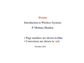
Errata Introduction to Wireless Systems P. Mohana Shankar • Page numbers are shown in blue • Corrections are shown in red March 2003
Page 11 below Figure 2.4 The power detected by a typical receiver is shown in Figure 2.5. Page 14 Expressing the frequency in MHz, eqn. (2.6) can now be expressed as where d must be larger than 1 km. The unit of f is in MHz and d is in kilometers. Page 17 top of the page to account for the terrain. Additional correction factors can be included to account for other factors such as street orientation. These correction factors They take into account the following: Page 13
Page 27 Figure 2.18 X axis label…, Envelope a or Power p Page 28 Sentence below eqn. (2.40) ………where p0 is the average power Page 15 Figure 2.7 Transmitted power = 100 mW instead of 100 dBm Page 19 Example 2. 3 Find approximate values of the loss parameter, n, using Hata model for the four geographical regions, namely large city, small-medium city, suburb, and rural area. Answer: Using Figure 2.12, the loss values at a distance of 3 km are 131.36 dB, 131.34 dB, 121.40 dB, and 102.8 dB, respectively, for large city, small-medium city, suburb, and rural area. Eqn. (2.40) Page 34 2.3.3 Frequency-dispersive Behavior of the Channel Page 39 2.3.5 Frequency dispersion vs Time dispersion We have seen that fading can be in the frequency domain or in the time domain. It is possible to treat the fading in wireless communications systems as constituted by independent effects. The channel shows time dispersive behavior when multipath phenomena are present. At the same time, independent of this effect, the channel will also exhibit frequency dispersion if the mobile unit is moving.
Signal bandwidth Page 39 Figure 2.31 Time dispersive/ frequency selective Slow and Frequency Selective Fast and Frequency Selective B c Time selective/ frequency dispersive Slow and Flat Fast and Flat T c Bit duration
0.7 Page 41 Figure 2.33 0.6 K = -¥ dB 0.5 K=6 dB K=14 dB K=18 dB 0.4 (a) A f 0.3 0.2 0.1 0 0 2 4 6 8 10 12 envelope a
Page 41 First sentence on top of the page The Rician probability density function is shown in Figure 2.33 for different values of the parameter K. Page 42 Eqn. 2. 66 Page 46 2.4.5 Summary of Fading The various fading mechanisms and the attenuation described can be summarized in a diagram shown in Fig. 2.38. Note that Rician and Rayleigh arise out of multipath effects and Nakagami can represent them both. This is not shown in the figure. For most of the cases, analyses based on Rayleigh or Rician fading are sufficient to understand the nature of the mobile channel. A number of recent publications (Alhu 1985, Anna 1998, 1999) have suggested the use of Nakagami fading models to provide a generalized view of fading in wireless systems. Page 53 Exercise 2.1 Using MATLAB, generate plots similar to the ones shown in Figure 2.7 to demonstrate the path loss as a function of the loss parameter for distances ranging from 2 Km to 40 Km. Calculate the excess loss (for values of n >2.0) in dB.
Page 54 Exercise 2.18. Generate a plot similar to the lognormal fading shown in Figure 2.36. Page 55 Exercise 2.17 Compare the maximum data transmission capabilities of the two channels characterized by the impulse responses shown below. (a) (b) FIGURE P2.17
P(f) f frequency 0 f - R f +R 0 0 |M(f)I2 0 R 2R frequency Page 75 Figure 3.18
Page 79 (below eqn. 3.45) The output noise, n(T), has a spectral density, Gout(f), given by (See Appendix A.6) Page 87 The probability of error can be expressed (Taub 1986) as (Exercise 3.21) Page 93 Table 3.2 DPSK encoding: Page 80 Eqn. (3.51) Use Min in place of Mout Page 90 The plot of error probability for different values of E/N0 (signal-to-noise ratio) is shown in Figure 3.28. Comparing eqn. (3.83) with the bit error rate for ASK systems (eqn. (3.79)), it is seen that the performance of a coherent BPSK is 3dB better than that of coherent ASK.
Data fn Page 94 In Figure 3.32, use xk and yk in place of Xk and Yk. 1 1 p/4 Page 98 -1 1 3p/4 -1 -1 1 -1 -3p/4 (or 5p/4) -p/4 (or7p/4) Table 3.4 Phase encoding in QPSK
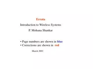
QPSK 1 0.5 0 -0.5 -1 0 1 2 3 4 5 6 7 8 1 0.5 0 -0.5 -1 0 1 2 3 4 5 6 7 8 Page 100 Figure 3.35 In Figure 3.35a, the line at 2 should be broken as shown. (a) QPSK (shifted by p /4) (b) amplitude time (units of T)
1 0.8 0.6 0.4 0.2 0 -0.2 -0.4 -0.6 -0.8 -1 0 1 2 3 4 5 6 7 Page 103 Figure 3.41 In the Figure the line at 1 should be broken as shown. amplitude time(units of T)
{-1 –1} Page 104 Figure 3.43
Page 125 As the number of levels of modulation increases, the minimum power required to maintain a fixed bit error rate decreases increases. This can be seen from the decision boundaries shown in Figure 3.71. cos[2p(f0+Df)t + S z 1 if z > 0 decision FSK (threshold = 0) 0 if z < 0 _ cos[2p(f0-Df)t Page 116 Figure 3.57 Page 124 Detection and Reception of MSK and GMSK Since MSK can be generated starting from OQPSK, the bit error performance of MSK will be identical to that of BPSK, QPSK or OQPSK. However, MSK and GMSK can also be detected using a 1-bit differential detector, 2-bit differential detector or a frequency discriminator. The block diagrams of these receiver structures are shown respectively in Figure 3.69 a, 3.69 b, and 3.69 c.
Figure 4.5 Frequency reuse pattern of cells. The alphabets (except D) represent the different channels. D is the distance between cells having the same frequency. Page 143 Figure 4.6 Expanded view of the cell structure showing a seven cell reuse pattern. H is the channel reused. Figure 4.7 A three-cell pattern (Nc=3)showing six interfering cells Page 141 Page 143 Because of this, q =D/R= is also known as the frequency reuse factor Page 143 TABLE 4.2 i j Nc q S/I(dB) Page 144
Eqn. 5.47) Page 169 Page 175 5.2.2 Effects of Frequency Selective Fading, Co-Channel Interference As discussed in Chapter 2, frequency selective fading arises when the coherent bandwidth of the channel is less than the message bandwidth. The error rates vary with the form of modulation and demodulation used. The performances of the modems also depend on the ratio of (sd/T), where sd is the r.m.s delay spread (eqn. 2.42) and T is the symbol period. The exact equations governing the error probability, taking frequency selective fading into account, are once again very complex, and are beyond the scope of this book. Numerical results are available in a number of research papers (Fung 1986, Guo 1990, Liu 1991a,b). Page 176 Figure 5.5 The legends should read dB instead of db. Page 189 The performances of the three signal processing schemes are shown in Figure 5.17, with gav equal to the signal-to-noise ratio after combining. They are also given in tabular form in Table 5.1. Page 195
Page 220 Page 214 First Paragraph Example 6.1 In a DS-CDMA cell, there are 24 equal power channels that share a common frequency band. The signal is being transmitted on a BPSK format. The data rate is 9600 bps. A coherent receiver is used for recovering the data. Assuming the receiver noise to be negligible, calculate the chip rate to maintain a bit error rate of 1e-3. Answer: Assuming that there is no thermal noise, the bit error rate is given by eqn. (6.15) where K is the processing gain and k is the number of channels. where Using the MATLAB function erfinv (.), we can solve for We get z = 4.77. We are given k=24; K=23*4.77=109.82. Since chip rate = 109.82*9600=1.05 Mchip/s. The PN sequence is unique to each user and is almost orthogonal to the sequences of other users. Thus, the interference from other users in the same band will be much less. The number of orthogonal codes, however, is limited. As the number of users increase, the codes become less and less orthogonal more and more correlated (orthogonality is compromised) and the interference will increase.
The radio capacity of the system, m, is defined as radio channels/cell. (6.21) Making use of the relationship between q and Nc (Chapter 4), , (6.22) Page 225 Figure 6.21 Block diagram of the transmitter associated with an AMPS system Changeto Page 231 Eqns. 6.21 and 6.22
Page 233 3rd line from the top Let us start by considering a single cell with N (= k of eqn (6.11)) users who share the cell. Page 233 Page 233 where R is the information bit rate and Bc is the RF bandwidth. We have divided the signal power (S) in the numerator by the bandwidth (data rate R) of the message data, while the signal power in the numerator has been divided by the bandwidth (Bc) occupied by the interfering signal. (See Section 3.2.7) The quantity (Bc /R) is the processing gain K of the CDMA processing, defined in connection with Figure 6.7. Page 234
Page 263 Normal or Gaussian distribution Page 250 Page 266 where G is the gamma function
![[Funded Programs Are Shown in Millions of Dollars]](https://cdn1.slideserve.com/2535390/slide1-dt.jpg)


![[Funded Programs Are Shown in Millions of Dollars]](https://cdn3.slideserve.com/6806993/slide1-dt.jpg)