3. Grey Modeling
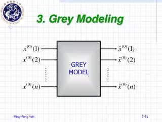
3. Grey Modeling. GREY MODEL. Grey Modeling. In grey system theory, a dynamic model with a group of differential equations called grey differential model is developed. A stochastic process whose amplitudes vary with time is referred to as a grey process ;

3. Grey Modeling
E N D
Presentation Transcript
3. Grey Modeling GREY MODEL
Grey Modeling • In grey system theory, a dynamic model with a group of differential equations called grey differential model is developed. • A stochastic process whose amplitudes vary with time is referred to as a grey process; • The grey modeling is based on the generating series rather than on the raw one; • The grey derivative and grey differential equation are defined and proposed in order to build a grey model; • To build a grey model, only a few data (as few as four) are needed.
Grey Model • Grey model, denoted by GM(n,h) model, is a dynamic model which consists of a group of grey differential equations, where n is the order of grey differential equations and h is the number of considered variables. • Grey models play an important role for the sequence (series) forecasting problem in the grey system theory. • Among all GM(n,h) models, the most commonly utilized grey model is the GM(1,1) model.
3.1: GM(1,1) Model • Let x(0) = {x(0)(1), x(0)(2),…, x(0)(n)} be a raw series and x(1) = AGO x(0), then x(0)(k) + az(1)(k) = b, k = 2,3,…,n. is a grey differential model. • This model is called GM(1,1) model since it consists only one variable. • z(1)(k) = 0.5x(1)(k) + 0.5x(1)(k-1), k = 2,3,…,n • a is the development coefficient. • b is the grey input.
GM(1,1) Model • Since x(0) = {x(0)(1), x(0)(2),…, x(0)(n)} and x(1) = {x(1)(1), x(1)(2),…, x(1)(n)} satisfy the GM(1,1) model, the following equations are held. • Error: , Cost function: • B is called a data matrix, yn is the data vector.
Solution of GM(1,1) Model • According to the least square method, we have • Another solution of a and b:
Whitened Equation • The whitened differential equations: • Initial value: x(0)(1) • Complete solution: • Let t = k + 1 • Predicted value:
Modeling Process • Take 1-AGO to original sequence x(0) • Construct the data matrix B and the data vector yn • Identify the development coefficient a and the grey input bby • Forecast the original sequence by
Exponential Law & Class Ratio • Let x(t) be a continuous function and c and a are constant, if x(t) = ceat, then x(t) satisfies the continuousexponential law. • Let x(t) be a continuous function and c, a and are constant, if x(t) = ceat+, then x(t) satisfies non-homogeneousexponential law. • Let x={x(1), x(2),…, x(n)}, the class ratio of series x at point k is defined as (k) = x(k-1)/x(k)
Class Ratio Let x={x(1), x(2),…, x(n)} • White class ratio: (k) = x(k-1)/x(k) = const, k • Non-homogeneous class ratio at point k: (k) = [x(k-1)x(k-2)]/[x(k)x(k-1)] If (k) = const, then the series x satisfies the non-homogeneouswhiteexponential law.
Class Ratio • Class ratio of r-AGO series x(r) (r)(k) = x(r)(k-1)/x(r)(k), k = 2,3,…,n; r = 0,1,2,… • If a series x(0) can be used to build a GM(1,1) model, the its class ratio must satisfy that
Example 3.1 • Let x(0)={79.8, 74, 61, 51} 1-AGO: x(1)={79.8, 153.8, 241.8, 265.8} z(1)={z(1)(2), z(1)(3), z(1)(4)}={116.8, 184.3, 240.3}
Equivalent Model 1 • x(0)(k) + az(1)(k) = b, z(1)(k) = 0.5x(1)(k) + 0.5x(1)(k-1), k = 2,3,…,n. • x(0)(k) = x(1)(k 1),k = 2,3,…,n. Proof: x(0)(k) + 0.5a[x(1)(k) +x(1)(k1)] = b x(1)(k) = x(1)(k1) + x(0)(k) [1+0.5a] x(0)(k) + a x(1)(k1) = b [1+0.5a] x(0)(k) = b a x(1)(k1)
Equivalent Model 2 • x(0)(k) + az(1)(k) = b, z(1)(k) = 0.5x(1)(k) + 0.5x(1)(k-1), k = 2,3,…,n. Proof: Formx(0)(k) = x(1)(k 1), k = 2,3,…,n, we have k = 2: x(0)(2) = x(1)(1) k = 3: x(0)(3) = x(1)(2) = [x(1)(1) + x(0)(2)] = (1 ) x(0)(2)
Equivalent Model 3 • x(0)(k) + az(1)(k) = b, z(1)(k) = 0.5x(1)(k) + 0.5x(1)(k-1), k = 2,3,…,n. • The forbidden region for a is (,2)(+2,). • If a = 2, then GM(1,1) model disappears. • If a = 2, then GM(1,1) model is meaningless.
3.2: Grey Series GM(1,1) • The first datum (1) is the grey number. • A GM(1,1) model built by above grey series has the following characteristic: 1. The developing coefficienta is independent of the first datum (1). 2. The predicted value is independent of (1). 3. The grey inputb is crucially dependent on (1). 4. The generating series is dependent on the grey number (1).
Grey Series GM(1,1) • To build a GM(1,1) model, the series must consist of at least four data. • If only three past data are available , then x(0)cannot be modeled. • However, then x(0)can be modeled and .
3.3: GM(1,N) Model • A grey differential equation having N variables is called GM(1,N) whose expression can be written as follows: where bi is said to be the ith influence coefficient which means that xi exercises influence on x1(the behavior variable).
GM(1,N) Model • Based on the least squared method, we have
GM(1,N) Model • The GM(1,N) whitened differential equation: • From the whitened differential eq., we have where
Example 3.3 • Original series: x1={134.8,148.2,145.3,146.6,154.4,153.7} x2={141.6,168.5,176.1,169.8,169.3,176.0} x3={152.8,173.2,203.0,214.2,221.1,244.1} x4={172.8,229.9,277.3,332.6,383.8,423.6} • Initializing ={1,1.0994,1.0778,1.0875,1.1454,1.1402} ={1,1.1899,1.2436,1.1991,1.1956,1.2429} ={1,1.1335,1.3285,1.4018,1.4469,1.5975} ={1,1.3304,1.6047,1.9247,2.2210,2.4513}
Example of GM(1,N) • By the Least Square Method, we have • From GM(1,N) model
GM(1,1) v.s. GM(1,N) • GM(1,1) model plays an important role in grey forecasting, grey programming and grey control. • GM(1,N) model has laid an important foundation for regional economic programming and grey multivariable control.CANNOT use to predict the considered sequences.