9.3 Taylor’s Theorem: Error Analysis for Series
130 likes | 347 Vues
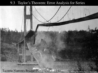
9.3 Taylor’s Theorem: Error Analysis for Series. Tacoma Narrows Bridge: November 7, 1940. Greg Kelly, Hanford High School, Richland, Washington.

9.3 Taylor’s Theorem: Error Analysis for Series
E N D
Presentation Transcript
9.3 Taylor’s Theorem: Error Analysis for Series Tacoma Narrows Bridge: November 7, 1940 Greg Kelly, Hanford High School, Richland, Washington
Taylor series are used to estimate the value of functions (at least theoretically - now days we can usually use the calculator or computer to calculate directly.) An estimate is only useful if we have an idea of how accurate the estimate is. When we use part of a Taylor series to estimate the value of a function, the end of the series that we do not use is called the remainder. If we know the size of the remainder, then we know how close our estimate is.
Use to approximate over . ex. 2: Since the truncated part of the series is: , the truncation error is , which is . For a geometric series, this is easy: When you “truncate” a number, you drop off the end. Of course this is also trivial, because we have a formula that allows us to calculate the sum of a geometric series directly.
Lagrange Form of the Remainder Taylor’s Theorem with Remainder If f has derivatives of all orders in an open interval I containing a, then for each positive integer n and for each x in I: Remainder after partial sum Sn where c is between a and x.
Note that this looks just like the next term in the series, but “a” has been replaced by the number “c” in . Lagrange Form of the Remainder This seems kind of vague, since we don’t know the value of c, but we can sometimes find a maximum value for . Remainder after partial sum Sn where c is between a and x. This is also called the remainder of order n or the error term.
If M is the maximum value of on the interval between a and x, then: Taylor’s Inequality Lagrange Form of the Remainder Note that this is not the formula that is in our book. It is from another textbook. This is called Taylor’s Inequality.
Taylor’s Inequality Prove that , which is the Taylor series for sinx, converges for all real x. ex. 2: Since the maximum value of sin x or any of it’s derivatives is 1, for all real x, M = 1. so the series converges.
On the interval , decreases, so its maximum value occurs at the left end-point. Find the Lagrange Error Bound when is used to approximate and . ex. 5: Remainder after 2nd order term
Taylor’s Inequality On the interval , decreases, so its maximum value occurs at the left end-point. error Find the Lagrange Error Bound when is used to approximate and . ex. 5: Error is less than error bound. Lagrange Error Bound
Euler’s Formula An amazing use for infinite series: Substitute xi for x. Factor out the i terms.
Let This is the series for cosine. This is the series for sine. This amazing identity contains the five most famous numbers in mathematics, and shows that they are interrelated. p