Download

1 / 73
730 likes | 738 Vues
M. Brown and D. Lowe, University of British Columbia. Recognising Panoramas. Introduction. Are you getting the whole picture? Compact Camera FOV = 50 x 35°. Introduction. Are you getting the whole picture? Compact Camera FOV = 50 x 35° Human FOV = 200 x 135°. Introduction.

E N D
M. Brown and D. Lowe, University of British Columbia Recognising Panoramas
Introduction • Are you getting the whole picture? • Compact Camera FOV = 50 x 35°
Introduction • Are you getting the whole picture? • Compact Camera FOV = 50 x 35° • Human FOV = 200 x 135°
Introduction • Are you getting the whole picture? • Compact Camera FOV = 50 x 35° • Human FOV = 200 x 135° • Panoramic Mosaic = 360 x 180°
Why “Recognising Panoramas”? • 1D Rotations () • Ordering matching images
Why “Recognising Panoramas”? • 1D Rotations () • Ordering matching images
Why “Recognising Panoramas”? • 1D Rotations () • Ordering matching images
2D Rotations (, ) • Ordering matching images Why “Recognising Panoramas”? • 1D Rotations () • Ordering matching images
2D Rotations (, ) • Ordering matching images Why “Recognising Panoramas”? • 1D Rotations () • Ordering matching images
2D Rotations (, ) • Ordering matching images Why “Recognising Panoramas”? • 1D Rotations () • Ordering matching images
Overview • Feature Matching • Image Matching • Bundle Adjustment • Multi-band Blending • Results • Conclusions
Outline Bundle Adjustmentand Multi-band Blending Feature Extraction Image Matching Input Images
Overview • Feature Matching • Image Matching • Bundle Adjustment • Multi-band Blending • Results • Conclusions
Overview • Feature Matching • SIFT Features • Nearest Neighbour Matching • Image Matching • Bundle Adjustment • Multi-band Blending • Results • Conclusions
Overview • Feature Matching • SIFT Features • Nearest Neighbour Matching • Image Matching • Bundle Adjustment • Multi-band Blending • Results • Conclusions
Invariant Features • Schmid & Mohr 1997, Lowe 1999, Baumberg 2000, Tuytelaars & Van Gool 2000, Mikolajczyk & Schmid 2001, Brown & Lowe 2002, Matas et. al. 2002, Schaffalitzky & Zisserman 2002
SIFT Features – Location Extrema of DoG Discard Low Contrast Discard Edge Points Output: x,y,σ Picture Credit: http://en.wikipedia.org/wiki/Scale-invariant_feature_transform
SIFT Features – Orientation • Difference of Gaussian Function: • G(x, y, kσ) = Gaussian Kernel with SD = kσ • L(x, y, kσ) = I(x, y) * G(x, y, kσ) • D(x, y, σ) = L(x, y, kiσ) – L(x, y, kjσ) • Gradient Magnitude: • m(x,y) = √{ (L(x + 1, y) – L(x - 1, y))2 + (L(x, y + 1) – L(x, y - 1))2 } • Θ(x, y) = tan-1{ (L(x, y + 1) – L(x, y - 1)) / (L(x + 1, y) – L(x - 1, y)) }
SIFT Features – Orientation Local Gradients Adjusted Gradients Gaussian Weighting Orientation Histogram – 36 bins with 10 degrees each
θ SIFT Features – Orientation Local Gradients Adjusted Gradients Gaussian Weighting Orientation Histogram – 36 bins with 10 degrees each
SIFT Features – Descriptor Vector • 4 x 4 region around point oriented according to θ • Take 8 versions of the gradient image corresponding to 8 different directions. • Each version has only gradients that fall in corresponding direction range • Concatenate the 8 versions (each 4 x 4) together to get 128 dimensional descriptor vector
SIFT Features • Invariant Features • Establish invariant frame • Maxima/minima of scale-space DOG x, y, s • Maximum of distribution of local gradients • Form descriptor vector • Histogram of smoothed local gradients • 128 dimensions • SIFT features are… • Geometrically invariant to similarity transforms, • some robustness to affine change • Photometrically invariant to affine changes in intensity
Overview • Feature Matching • SIFT Features • Nearest Neighbour Matching • Image Matching • Bundle Adjustment • Multi-band Blending • Results • Conclusions
Nearest Neighbour Matching • Find k-NN for each feature • k number of overlapping images (we use k = 4) • Use k-d tree • k-d tree recursively bi-partitions data at mean in the dimension of maximum variance • Approximate nearest neighbours found in O(nlogn)
Overview • Feature Matching • SIFT Features • Nearest Neighbour Matching • Image Matching • Bundle Adjustment • Multi-band Blending • Results • Conclusions
Overview • Feature Matching • Image Matching • Bundle Adjustment • Multi-band Blending • Results • Conclusions
Overview • Feature Matching • Image Matching • Bundle Adjustment • Multi-band Blending • Results • Conclusions
Overview • Feature Matching • Image Matching • RANSAC for Homography • Probabilistic model for verification • Bundle Adjustment • Multi-band Blending • Results • Conclusions
Overview • Feature Matching • Image Matching • RANSAC for Homography • Probabilistic model for verification • Bundle Adjustment • Multi-band Blending • Results • Conclusions
Homography Defn – Homography: A one-to-one mapping between two images. In computer vision, it is typically used to describe the correspondence between two images taken of the same scene from different camera angles. For Images: Homography has four parameters, θ1θ2θ3 f, corresponding to the three angles of camera rotation and the focal length. Picture Credit: http://weboflife.nasa.gov/learningResources/vestibularbrief.htm
RANSAC(RANdom SAmple Consensus) bestH = 0% success While i < max iterations: - Select a random sample of the data - currentH = solve for the homography using sample data - for each pair of points, test to see if currentH is a suitable solution - if more points work with currentH than with bestH set bestH = currentH
Overview • Feature Matching • Image Matching • RANSAC for Homography • Probabilistic model for verification • Bundle Adjustment • Multi-band Blending • Results • Conclusions
Probabilistic model for verification • Want to solve for the probability that the image match is correct given the set of RANSAC inliers and outliers. • p( match | inliers ) • Using Bayes’ Rule: • p( match | inliers ) = p( inliers | match ) * p( match ) / p( inliers ) • This can be simplified if we make some assumptions • p( inliers | match ) = B( ni; nf, p1) • p( inliers | ~match ) = B( ni; nf, p0) (B is a binomial distribution function)
Probabilistic model for verification • Compare probability that this set of RANSAC inliers/outliers was generated by a correct/false image match • ni = #inliers, nf = #features • p1 = p(inlier | match), p0 = p(inlier | ~match) • pmin = acceptance probability • Choosing values for p1, p0 and pmin
Overview • Feature Matching • Image Matching • RANSAC for Homography • Probabilistic model for verification • Bundle Adjustment • Multi-band Blending • Results • Conclusions
Overview • Feature Matching • Image Matching • Bundle Adjustment • Multi-band Blending • Results • Conclusions
Overview • Feature Matching • Image Matching • Bundle Adjustment • Multi-band Blending • Results • Conclusions
Bundle Adjustment • Overlay the images together one at a time. • For each image, solve for the camera parameters θ1θ2θ3 f to align it with the current compilation using Levenberg-Marquardt to minimize an error function.
Overview • Feature Matching • Image Matching • Bundle Adjustment • Error function • Multi-band Blending • Results • Conclusions
Overview • Feature Matching • Image Matching • Bundle Adjustment • Error function • Multi-band Blending • Results • Conclusions