A Survey on the Tree augmentation problem
570 likes | 591 Vues
Survey and analysis of the tree augmentation problem in graph theory, covering concepts like laminar families, shadow completion, and LP-based solutions with approximation ratios. The text presents key findings, notable approaches, and unresolved challenges in the field.

A Survey on the Tree augmentation problem
E N D
Presentation Transcript
A Survey on the Tree augmentation problem Guy Kortsarz
Augmenting edge connectivityfrom 1 to 2 Given: undirected graph G(V,E) and a set of extra legal for addition edges F with cost c(e) for every edge e Required: a subset F’ F of minimum cost so that G(V,E+F’) is 2-edge-connected
Bi-Connected Components G A H F B D E C
The tree augmentation problem Input: A tree T(V,E) and a separate set edge F with cost on every link Output: Add minimum cost set of links F’ from F so there will be no bridges (G+F’ is 2EC)
Another way of posing the problem • A family of sets is laminar is for any two set A,B, either one set contains the other or the sets are disjoint. • A laminar family is a tree. So our problem is equivalent to covering Laminar families • Part of a subject to know: uncrossing.
Uniform versus non-uniform weights • TAP admits a ratio 2 approximation, that can be derived by the Jain method GW primal dual method and by other techniques • We start with the uniform costs case since is seems to be easier to approximate. • For uniform, better than 2 ratio known for a while.
Shadow Completion • Part of the shadows added
Shadows-Minimal Solutions • If a link in the optimum can be replaced by a proper shadow and the solution is still feasible, do it. • Claim: in any SMS, the leaves have degree 1
Covering minimally leaf-closed trees • Let up(l)be the “highest link” (closest to the root) for l, after shadow completion. • Let T’ be a minimally leaf-closed tree • Then {up(l) | lT } covers T’ • Given that, we spent L links in covering T’. The optimum spent at least L/2 • A ratio of 2 follows
Proof • If an edge eT’ is not covered then we found a smaller leaf-closed tree T’’ e T’’ v
Approximation ratios for the uniform cost case • First to break the ratio of 2 was Nagamochi. About 40 pages paper. Ratio roughly 1.9. DAM • In 2016 after 15 years of simplifications, K, Nutovgave 1.5 ratio (combinatorial) TALG 2016. • Cheriyan and Gao gave the same ratio with similar algorithm but novel analysis
Continued • Cheriyan et al used Lift and Project to prove the 3/2 ratio. Interesting idea: proving ratio of a combinatorial algorithm by Lift and Project. Algorithmica 2018 • Best known approximation ratio 1.458 by Grandoni Kalaitzis Zenklusen. • LP based. STOC 2018.
What do we know on the basic LP? • link j covers edge exj ≥1, xj ≥0 • J. Cheriyan H. Karloff R. Khandekar J. ̈Konemann. 3/2IG. • The two in green are now working in Wall Street. • Nutov: IG at most2-2/15.
Any solution has a matching on the leaves • Therefore it is natural to find a maximum matching on the leaves. Every combinatorial algorithm does just that. Except for the dual fitting of K. Nutov that finds a maximal matching. • What about an algorithm that finds a maximum matching, contract and iterate? Not better than 2.
Problematic structure: Stem • A link whose contraction creates a leaf STEM Twin Link
How to design a lower bound trivially • Say we want a 3/2 ratio. • Consider OPT • Each leaf to leaf link in OPT gets 3/2 units and each unmatched leaf has 3/2. • But the other end of the unmatched link is not a leaf. Transfer ½ from the unmatched leaf to the non leaf leaving credit 1 for unmatched leaf.
We do not know the optimum • So we do it with a maximum matching • Easy to see: each matched link credit 3/2 and each unmatched credit 1, and stem link credit 2 is a lower bound. • Because our matching can only be larger.
Problematic structure: Stem • A link whose contraction creates a leaf 3/2+1/2=2 STEM 1 Twin Link
Main idea • Find a tree with k+1 credit that can be covered with k links • Leave 1 unit on the root. 1 K+1
Problematic structure: Stem • Since stem link has credit 2 add link and leave 1. STEM Twin Link
We cover a tree similar to Minimally Leaf Closed. • Minimally leaf closed means that links touching the leaves do not go outside the tree, and the tree is minimal with respect to this property. • We need 1 to take matched links so ½ spare. • Two matched pairs give extra credit 1. • Put 1 on the the new leaf. • Difficulty: trees with one matched pair.
Integrality gap of better than 2: for the unweighted case. • If the twin link is taken then there is a link to the stem with the same value. STEM Twin Link
First IG better than 2, was for uniform costs K,Nutov • K. Nutov. Include the mentioned valid inequality, without whom, we could not show any integrality gap better than 2. • The more interesting algorithm that shows 7/4 integrality gap is a dual fitting. We do not need to solve an LP • In fact we only need to find a maximal matching. Very fast algorithm.
The weighted case: no leaf closed trees • We may assume it’s a metric, since the problem on a path is polynomial. • Cheriyan Jordan and Ravi: the problem is hard even if the links are an Hamiltonian path on the leaves. • A ½ integral solution gives 4/3 ratio. • But in most cases not half integral.
The weighted case: no leaf closed trees • If the diameter is constant then there is a better than 2 ratio: 1+ln 2 in time nf(D)Cohen and Nutov. • Landau and Nutov: study the case links are leaf to leaf. • The problem parametrize by opt is fixed parameter tractable. • Due to Marx et al
Perhaps the simplest idea to get a ratio 2 for TAP. • If all the links inside principal trees are up links (from an ancestor to a descendant) then we get that the Matrix is totally unimodular • This means that Basic Feasible Solution has integral entries. • Double an link (u,v). Say that w is the LCA, change to (u,w) (v,w)
Lin : links inside principal trees • Let optin be the cost of LinOPT • Let optcrbe the rest of the optimum. • Note that the trivial algorithm gives a solution of cost optcr +2optin • Only if optinhas almost all the cost would this be a ratio 2.
A significant breakthrough • We were surprised by a paper of Adjiashvili that gave a 1.96 ratio for TAP if the maximum weight is bounded by a constant. • The paper had a truly original approach and many pretty ideas. • For uniform cost gave 5/3 LP based. Improving K,Nutov 7/4
Some remarks • We root the tree at a vertex r. • Make sure no edge is covered by more than 2/flow. • Denote by M the maximum cost of a link covered by at most 2/ • Thus every edge is covered by at most 2M/cost.
Some more definitions • The trees rooted at childrens of r are called principal trees. • Also, a principal tree is called heavy if the LP cost inside the tree (links both of its endpoints are in the principal tree) is at least 2M/2 • We only separate heavy trees from the input tree.
An Overview • Principal trees are trees rooted at the children of the root r. • Principal edges are edges from the root to a child. • Divide and conquer: remove heavy trees.
Overview • Principal trees are trees rooted at the children of the root r. • Principal edges are edges from the root to a child. • Divide and conquer:
How to keep the LP legal: cut at shadows • LP is legal afte we cut at shadows.
The trees now do not contain all edges • We need to explain how we cover with negliable cost edges that are removed by the divide and conquer. • Namely, principal edges from the root to a child that roots a heavy tree. • We use the fact that we separated only heavy trees.
Say that we deleted k heavy trees • Since every edge is covered by at most 2/and M is the maximum cost covering these k trees costs at most 2Mk/ • Since every removed tree is heavy, the cost of separated trees is at least 2Mk/2 • Hence in total we pay at most opt
After iteratively divide and conquer • The principal trees that remain are all of low cost, namely at most 2Mk/2 cost. • Every link has a cost of at least 1 • Thus the number of leaves in every principal tree is at most 2Mk/2 • This is constant, since M is.
Dealing with principal trees of constant cost • This case is divides into two sub cases • Depending on if the crossing links are fractionally heavier. In this case we reduce to a well known problem: Edge cover. • Or the internal links are fractionally heavier. Solve optimally each small tree by exhaustive search.
The internal fraction is smaller • Say that the fractional cost of cross edges is more than the cost of edges between principal trees. Consider only cross edges. • The vertex r belongs to all the covering paths. This is equivalent to Edge Cover of the leaves. The basic LP gives a 4/3 approximation.
The second case • We can compute the optimum of tree rooted at a child in polynomial time. • We make sure that the LP is at least the integral optimum. • It’s a valid inequality. The LP should have value at least opt because OPT is a valid solution. This is almost never used since we almost never know opt.
People may have thought • The 4/3 factor should be removed. • No need to solve optimally on small forests. Trees will do. • Adding the odd cut inequalities is highly natural (makes the Edge Cover integral). • We discuss the work of Fiorini, Groß, Könemann, and Sanità
Adding some known inequalities • The {0,1/2} Chvatal Gomory cut inequalities. Algebra based inequalities. • In general separation is NP-Hard. • But in this case a (non trivial) proof shows that the that this is reduced to adding odd cut inequalities. • Can be separated in poly time.
Edge cover of odd size sets U • The odd cut inequality: the number of links touching U required to cover U is at least (|U|+1)/2 • If you add all the odd cut inequalities then the solution for Edge Cover is integral. • Its not trivial to combine the ideas.
Remove all crossing edges • We are talking on the case that internal links dominate. • The authors suggested two things: remove all crossing links. • This increases the cost: 2optcr +optin • The crossing edges have been replaced by up edges. Fiorini et al show: in this case the BFS are integral.
How does the 3/2+ follow • Always known optcr+2optin • The sum of 2optcr+optin and optcr+2optin is 3optcr+3optin • Thus one of the two solutions has cost 3opt/2 ratio. In fact: • A 3/2+ is the right ratio because we deleted heavy trees.
Based on this paper • Nutov gave an exp(M,1/) time to solve the problem when the trees are small. • Because Nutov showed that it is enough to solve the bundle inequalities on trees. Not on forests. • The ratio is the same, namely 3/2+ • However given the time to solve optimally the case of small trees, the ratio works for M=O(log n)