Instructions for Converting POLYMATH Solutions to Excel Worksheets - Introduction
530 likes | 663 Vues
This guide outlines the process for converting POLYMATH solutions into Excel worksheets, specifically focusing on numerical problem-solving relevant to chemical engineering. It emphasizes the benefits of using Excel for computational tasks and provides detailed instructions on converting various types of problems, including nonlinear algebraic equations, systems of equations, and regression analyses. Step-by-step methods are outlined for utilizing Excel's Goal Seek and Solver tools, enhancing the engineer's ability to modify and document models efficiently.

Instructions for Converting POLYMATH Solutions to Excel Worksheets - Introduction
E N D
Presentation Transcript
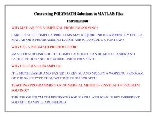
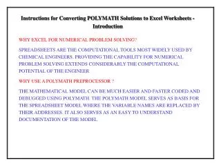
Instructions for Converting POLYMATH Solutions to Excel Worksheets - Introduction WHY EXCEL FOR NUMERICAL PROBLEM SOLVING? SPREADSHEETS ARE THE COMPUTATIONAL TOOLS MOST WIDELY USED BY CHEMICAL ENGINEERS. PROVIDING THE CAPABILITY FOR NUMERICAL PROBLEM SOLVING EXTENDS CONSIDERABLY THE COMPUTATIONAL POTENTIAL OF THE ENGINEER WHY USE A POLYMATH PREPROCESSOR ? THE MATHEMATICAL MODEL CAN BE MUCH EASIER AND FASTER CODED AND DEBUGGED USING POLYMATH. THE POLYMATH MODEL SERVES AS BASIS FOR THE SPREADSHEET MODEL WHERE THE VARIABLE NAMES ARE REPLACED BY THEIR ADDRESSES. IT ALSO SERVES AS AN EASY TO UNDERSTAND DOCUMENTATION OF THE MODEL
1 ONE NONLINEAR ALGEBRAIC EQUATION – GOAL SEEK – SLIDES 3-9 2 SYSTEMS OF NONLINEAR ALGEBRAIC EQUATIONS – SOLVER – SLIDES 10-14 3 ODE – INITIAL VALUE PROBLEMS – 4TH ORDER EXPLICIT RK – SLIDES 15-24 4 ODE – BOUNDARY VALUE – EXPLICIT EULER + GOAL SEEK – SLIDES 25-29 5 DAE – INITIAL VALUE PROBLEMS – IMPLICIT EULER – SLIDES 30-36 6 PDE – INITIAL VALUE - METHOD OF LINES – EXPLICIT EULER – SLIDES 37-40 7 MULTIPLE LINEAR REGRESSION – LINEST – SLIDES 41-45 8 POLYNOMIAL REGRESSION – LINEST – SLIDES 46-49 9 MULTIPLE NONLINEAR REGRESSION – SOLVER – SLIDES 50-53 CONVERTING POLYMATH SOLUTIONS TO EXCEL WORKSHEETS TYPES OF PROBLEMS DISCUSSED
One Nonlinear Algebraic Equation Instructions for Conversion (1) To obtain a basic solution of a system containing one implicit nonlinear algebraic equation and several explicit equations the POLYMATH equations should be converted to Excel formulas and then the "Goal Seek" tool can be used. In order to obtain a well documented Excel worksheet, which can be easily modified for parametric runs it is recommended to carry out the conversion in the following steps: 1. Copy the implicit equation and the ordered explicit equations from the POLYMATH solution report. 2. Paste the equations into an Excel worksheet; remove the text and the equation numbers. 3. Rearrange the equations in the order: constant definitions, functions of the constants, parameter definitions, unknown, explicit functions of the unknown and implicit function of the unknown.
One Nonlinear Algebraic Equation Instructions for Conversion (2) 4. Copy the right hand side of the equations into the adjacent cell and replace the variable names by variable addresses. Note that "If" statements and some functions may require additional rewriting and/or rearrangement. Use absolute addressing for the constants and the functions of constant and relative addressing for the unknown and its functions (Note that pressing F4 converts selected reference from relative to absolute). In the cell adjacent to the unknown put its initial estimate. 5. Use the "Goal Seek" tool to set the value of the cell containing the implicit function of the unknown at zero while changing the value in the cell of the unknown..
One Nonlinear Algebraic Equation Ordered POLYMATH File The use of this procedure is demonstrated in reference to Demo 2. Nonlinear equations [1] f(V) = (P+a/(V^2))*(V-b)-R*T = 0 Explicit equations [1] P = 56 [2] R = 0.08206 [3] T = 450 [4] Tc = 405.5 [5] Pc = 111.3 [6] Pr = P/Pc [7] a = 27*(R^2*Tc^2/Pc)/64 [8] b = R*Tc/(8*Pc) [9] Z = P*V/(R*T)
One Nonlinear Algebraic Equation Excel Formulas
One Nonlinear Algebraic Equation Solution To solve the nonlinear equation in cell C15 "Goal Seek" is used to set the value in this cell at zero while changing the contents of cell C13.
One Nonlinear Algebraic Equation Modifying the Equation Set The example is next solved for Pr = 1, 2, 4, 10 and 20. To achieve this, the parameter Tr and its function P=Pr*Pc are added to the equation set and the cells containing the unknown and its functions are copied and modified as necessary.
One Nonlinear Algebraic Equation Complete solution set To obtain the solution for other values of Pr cells 24 – 27 of column C are copied and the value of Pr entered in row 23. "Goal Seek" is applied separately to every column containing a different Pr value.
Systems of Nonlinear Algebraic Equations Instructions for Conversion (1) To obtain a basic solution of a system containing several implicit nonlinear algebraic equations the POLYMATH equations are converted to Excel formulas and then the "Solver" tool is used.The recommended steps for conversion are: 1. Copy the implicit equations and the ordered explicit equations from the POLYMATH solution report. 2. Paste the equations into an Excel worksheet; remove the text and the equation numbers. 3. Rearrange the equations in the order: constant definitions, functions of the constants, parameter definitions, unknowns, explicit functions of the unknowns and implicit functions of the unknowns. 4. Add an equation with the sum of squares of the implicit functions.
Systems of Nonlinear Algebraic Equations Instructions for Conversion (2) 5. Copy the right hand side of the equations into the adjacent cell and replace the variable names by variable addresses. Use absolute addressing for the constants and the functions of constant and relative addressing for the unknowns and functions of the unknowns. In the cell adjacent to the unknowns put initial estimates. 6. Use the "Solver" tool to set the value of the cell containing the sum of squares of the implicit functions of the unknowns at zero (or minimizing its value) while changing the values in the cells of the unknowns.
Systems of Nonlinear Algebraic Equations Ordered POLYMATH File The use of this procedure is demonstrated in reference to Demo 5 Nonlinear equations [1] f(CD) = CC*CD-KC1*CA*CB = 0 [2] f(CX) = CX*CY-KC2*CB*CC = 0 [3] f(CZ) = CZ-KC3*CA*CX = 0 Explicit equations [1] KC1 = 1.06 [2] CY = CX+CZ [3] KC2 = 2.63 [4] KC3 = 5 [5] CA0 = 1.5 [6] CB0 = 1.5 [7] CC = CD-CY [8] CA = CA0-CD-CZ [9] CB = CB0-CD-CY
Systems of Nonlinear Algebraic Equations Excel Formulas The "Solver" tool is used to minimize the sum of squares of errors in cell C20 by setting C20 as "target cell" and searching for its minimal value by changing cells C10, C11 and C12.
ODE – Initial Value Problems The Runge-Kutta Method There are no tools in Excel to solve differential equations so the solution algorithm must be build into the solution worksheet. In this example a fixed step size, explicit, fourth-order Runge-Kutta algorithm is used. The system of N first-order ODE for the functions is written : (1) The fourth-order Runge-Kutta formula is written: (2) This formula advances a solution from xnto
ODE – Initial Value Problems Instructions for Conversion (1) Apply the Runge-Kutta algorithm to the system of first-order, ODE carry out the conversion from the POLYMATH file to the Excel spreadsheet in the following steps: 1.Copy the differential equation and the ordered explicit algebraic equations from the POLYMATH solution report. 2. Paste the equations into an Excel worksheet; remove the text and the equation numbers. 3. Put the parameters: final value of the independent variable and integration step-size (h) in the first cells of the worksheet. Rearrange the equations in the order: constant definitions, functions of the constants,independent variable,dependent variables, explicit functions of the variables and differential equations.
ODE – Initial Value Problems Instructions for Conversion (2) 4. Copy the right hand side of the equations into the adjacent cell and replace the variable names by variable addresses. Use absolute addressing for the constantsand the functions of constant and relative addressing for the variables and functions of the variables. In the cell adjacent to the variables put their initial values. 5. Copy the section starting with the independent variable up to the end of the equation set and paste this section three times below, to obtain the values of k2, k3 and k4. Change the equations as needed to reflect the change in the variable values, as shown in Equation (2). 6. In the next column write the equations to calculate the advanced values of the independent and dependent variables. 7. Copy and paste the columns (or rows) as many time as needed in order to reach the final value of the independent variable.
ODE – Initial Value Problems Ordered POLYMATH File The use of this procedure is demonstrated in reference to Demo 9. Differential equations as entered by the user [1] d(T1)/d(t) = (W*Cp*(T0-T1)+UA*(Tsteam-T1))/(M*Cp) [2] d(T2)/d(t) = (W*Cp*(T1-T2)+UA*(Tsteam-T2))/(M*Cp) [3] d(T3)/d(t) = (W*Cp*(T2-T3)+UA*(Tsteam-T3))/(M*Cp) Explicit equations as entered by the user [1] W = 100 [2] Cp = 2.0 [3] T0 = 20 [4] UA = 10. [5] Tsteam = 250 [6] M = 1000
ODE – Initial Value Problems Excel Formulas (2)
ODE – Initial Value Problems Excel Formulas (3) In column D the solution isadvanced from xnto
ODE – Initial Value Problems Results for t=1 min and t=80 min (1)
ODE – Initial Value Problems Results for t=1 min and t=80 min (2)
ODE – Initial Value Problems Plot of the results
ODE – Boundary Value Problems Solution Method There are no tools in Excel to solve differential equations so the solution algorithm must be build into the solution worksheet. In this example a fixed step size, explicit, Euler algorithm is used. After setting up the worksheet for integrating the differential equations the "Goal Seek" (for the case of one boundary value) or the "Solver" (for the case of several boundary values) is used for converging to the proper initial values. The formula for the Euler method is (3) This formula advances a solution from xnto Steps of the Solution. 1. Copy the differential equation and the ordered explicit algebraic equations from the POLYMATH solution report. 2. Paste the equations into an Excel worksheet; remove the text and the equation numbers.
ODE – Boundary Value Problems Steps of the Solution 3. Put the parameters: final value of the independent variable and integration step-size (h) in the first cells of the worksheet. Rearrange the equations in the order: constant definitions, functions of the constants, independent variable, dependent variables, explicit functions of the variables and differential equations. 4. Copy the right hand side of the equations into the adjacent cell and replace the variable names by variable addresses. In the cell adjacent to the variables put their initial values. If the initial value is not known put initial estimates, instead. 5. In the next column write the equations to calculate the advanced values of the variables using Equation 3. 6. Copy and paste the columns as many times as needed in order to reach the final value of the independent variable. 7. Use the "Goal Seek" (for the case of one boundary value) or the "Solver" (for the case of several boundary values) to converge to the desired final value of the variables while changing their initial values.
ODE – Boundary Value Problems POLYMATH File and Excel Formulas The use of this procedure is demonstrated in reference to Demo 8. Differential equations as entered by the user [1] d(CA)/d(z) = y [2] d(y)/d(z) = k*CA/DAB Explicit equations as entered by the user [1] k = 0.001 [2] DAB = 1.2E-9
ODE – Boundary Value Problems • Results at z = 0, 0.00001 and 0.001 m • 1. Initial estimate: y = -150 • 2. After using of the "Goal Seek" tool to set the value of y(0.001) at zero while changing y(0).
DAE – Initial Value Problems Solution Method There are no tools in Excel to solve differential equations so the solution algorithm must be build into the solution worksheet. In this example a fixed step size, implicit, Euler algorithm is used. Using this method the differential equations are converted into nonlinear algebraic equations. Thus, in each integration step a system of nonlinear algebraic equations is solved using the "Solver" tool. The formula for the implicit Euler method is (4) This formula advances a solution from xn-1to for n>1.
DAE – Initial Value Problems Steps of the Solution (1) 1. Copy the differential equations and the ordered explicit algebraic equations from the POLYMATH solution report. 2. Paste the equations into an Excel worksheet; remove the text and the equation numbers. 3. Put the parameters: final value of the independent variable and integration step-size (h) in the first cells of the worksheet. Rearrange the equations in the order: constant definitions, functions of the constants, independent variable, dependent variables, explicit functions of the variables, differential equations and implicit algebraic equations. 4. Add an equation with the sum of squares of the implicit functions (the algebraic equations and the implicit Euler method representation of the differential equations).
DAE – Initial Value Problems Steps of the Solution (2) 5. Copy the right hand side of the equations into the adjacent cells and replace the variable names by variable addresses. Use absolute addressing for the constants and the functions of constant and relative addressing for the variables and functions of the variables. In the cell adjacent to the variables put their initial values. In the cell containing the sum of squares of the function values include only the functions associated with the implicit algebraic equations. 6. Use the "Solver" (or "Goal Seek" tools) to find the initial values of the unknowns associated with the implicit algebraic equations. 7. In the next column write the equations to calculate the advanced values of the independent and dependent variables. 8. From this point on the columns can be copied and pasted, as many time as needed to reach the final value of the independent variable. The "Solver" tool must be applied on the columns sequentially, to solve the system of nonlinear algebraic equations for each step
DAE – Initial Value Problems POLYMATH File The use of this procedure is demonstrated in reference to Demo 11 The differential equations and the ordered explicit algebraic equations as copied from the POLYMATH solution report are the following. Differential equations as entered by the user [1] d(L)/d(x2) = L/(k2*x2-x2) [2] d(T)/d(x2) = Kc*err Explicit equations as entered by the user [1] Kc = 0.5e6 [2] k2 = 10^(6.95464-1344.8/(T+219.482))/(760*1.2) [3] x1 = 1-x2 [4] k1 = 10^(6.90565-1211.033/(T+220.79))/(760*1.2) [5] err = (1-k1*x1-k2*x2)
DAE – Initial Value Problems Excel formulas In the next column (column D)the definition of the independent variable is changed to: =C8+$C$7 and the definition of the sum of squares of errors is changed to: =(D9-(C9+($C$7/2)*(C14+D14)))^2+D15^2 .
DAE – Initial Value Problems Results for x2 = 0.4 and 0.42 Results obtained by applying "Goal Seek" to set cell C15 at zerowhile changing the initial temperature (cell C10) and subsequently applying the "Solver" tool to minimize the value in cell D16 while changing the contents of cells D9 and D10.
DAE – Initial Value Problems Results for x2 = 0.8 Column D is copied and pasted as many time as necessary to reach the final value of x2 (= 0.8). The "Solver" tool is applied sequentially, for every column to minimize the value in row 16.
Partial Differential Equations Excel Formulas for Demo 12 (1) The system of PDEs is converted into a system of first order ODEs using the method of lines. Explicit Euler's method is used for solution.
Partial Differential Equations Excel Formulas for Demo 12 (2) Column D for this section is obtained by copying and pasting the same section in column C. To obtain the complete solution column D is copied and pasted as many times as needed for reaching the final time.
Partial Differential Equations Results for t=0, 30 and 6000 min
Partial Differential Equations Plot of Some Results for Demo 12
Multiple Linear Regression Copying the Data from POLYMATH In this demonstration Riedel's equation is fitted to the data of Demo 6.
Multiple Linear Regression Pasting the Data into Excel and Adding Titles
Multiple Linear Regression Using the LINEST Function The LINEST function puts the full set of results in an area that includes 5 rows and number of columns as the number of the parameters. For this problem mark an area of 5 rows and 4 columns. Type in LINEST(D2:D11, A2:C11, TRUE,TRUE) and press CONTROL+SHIFT+ENTER to enter this formula into all the marked cells. Note that the range D2:D11 is the range where the dependent variable values are stored, the range A2:C11 is the range where the independent variable values are stored, the first logical variable TRUE (or the number 1) indicates that the parameter a0cannot be assumed to be zero and the second logical variable TRUE indicates that a matrix of regression statistics should also be returned. It is permitted to mark a one-, two-, three-, four-, or five-row array depending on the amount of information desired. The results obtained do not include any labeling and labeling should be added manually.
Multiple Linear Regression Results (1) For obtaining the results reported by POLYMATH the first three rows are significant. The first row (coeff.s) contains the values of the parameters. The second row (std. dev. S.) contains the standard deviation of the parameters. These values can be multiplied by the appropriate value from the t distribution to obtain the 95% confidence intervals. The square of the standard error in y (SE y) is the variance as reported by POLYMATH.
Multiple Linear Regression Variance and Confidence intervals and Residuals Removing the extra rows from the results table and adding the calculations of the confidence intervals and the variance yields the following table (only the first two columns out of the four are shown). Note that the t value for 95% confidence intervals with 6 degrees if freedom is: t = 2.4469.
Polynomial Regression Options and Instructions The LINEST function and "Regression" tool from the "Analysis ToolPak" can be used for carrying out linear regression. The LINEST function has the advantages over the "Regression" tool that the calculation results are automatically updated when the data is modified and the results are easier to rearrange for documentation purposes. The "Regression" tool provides more statistical data and the output is clearly labeled. The use of the LINEST function for carrying out polynomial regression will be demonstrated here in reference to Problem 2.3a in the book of Cutlip and Shacham. To prepare the data file arrange the columns of data so that the column of the dependent variable and the column of the independent variable are next to each other and put the column of the independent variable as the last one. Copy these columns of the data from the POLYMATH data table and paste them into an Excel worksheet. Define additional columns that contain increasing powers of the independent variable, up to the 5th degree.
Polynomial Regression Excel Formulas and Numerical Values Numerical values
Polynomial Regression Using the LINEST Function for a 2nd Degree Polynomial To solve for a second order polynomial (with three parameters) mark an area of 3 rows and 3 columns. Type in LINEST(A2:A20, B2:C20, TRUE,TRUE) and press CONTROL+SHIFT+ENTER to enter this formula into all the marked cells. Note that the range A2:A20 is the range where the dependent variable values are stored, the range B2:C20 is the range where the independentvariablevalues are stored, the first logical variable TRUE (or the number 1) indicates that the parameter a0 cannot be assumed to be zero and the second logical variable TRUE indicates that a matrix of regression statistics should also be returned. The results obtained do not include any labeling and labeling is added manually.
Polynomial Regression Results for a 2nd Degree Polynomial Calculation of the confidence intervals and the variance (only the first two columns out of the four are shown).
Multiple Nonlinear Regression Instructions To carry out multiple nonlinear regression an objective function containing the sum of squares of the errors is prepared and this objective function is be minimized by means of the "Solver" tool by changing the regression model parameters. Demo 6c is used as an Example. In this particular example the Antoine equation is fitted to vapor pressure (Vp) versus temperature (T °C) data. Thus, the objective function to be minimized is the following. (5) After copying the independent and dependent variable data from the POLYMATH file and pasting them into an Excel worksheet the objective function can be calculated in three successive columns.