Download
1 / 32
320 likes | 491 Vues
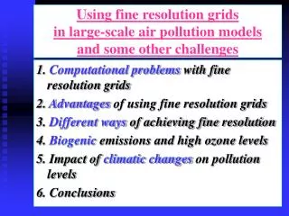
Using fine resolution grids in large-scale air pollution models and some other challenges. 1. Computational problems with fine resolution grids 2. Advantages of using fine resolution grids 3. Different ways of achieving fine resolution 4. Biogenic emissions and high ozone levels

E N D
Using fine resolution grids in large-scale air pollution modelsand some other challenges 1. Computational problems with fine resolution grids 2. Advantages of using fine resolution grids 3. Different ways of achieving fine resolution 4. Biogenic emissions and high ozone levels 5. Impact of climatic changes on pollution levels 6. Conclusions
Major requirements • More details about the pollution levels in Europe • More reliable information about trends and relationships concerning of the pollution levels over a long time-interval Great challenges for the modellers
Some of the major challenges • High resolution computations: lead to huge computational tasks • Taking into account all relevant factors (biogenic emissions can be mentioned as an example): leads to long series of runs with different scenarios • Impact of climatic changes on high pollution levels: leads to long-term runs (and, again, many scenarios are needed)
UNI-DEM Parameter Allowed values Desirable features NX 96, 288, 480 more possibilities NY NY=NX rectangular domains NZ 1, 10 more layers NS 35, 56, 168 RADM2, RACM NEMIS 0, 1 more flexibility NCHUNKS used in parallel runs NYEAR 1989-1998 data for more years
Computational difficulties Grid 96x96x10 480x480x10 Species 35 35 Equations 3 225 600 80 640 000 Time-steps 35 520 213 120 Processors 32 32 CPU hours 2.48122.83 Running UNI-DEM for 1997
Impact of the biogenic VOC emissions • Why are studies related to the impact of biogenic emissions on high ozone levels important? 1. The relative part of the biogenic emissions (related to the total VOC emissions) is increased, because the human made emissions were decreased during the last 10-15 years. 2. The relative part of the biogenic emissions in the summer months is even more increased, because a great part of these emissions is emitted during this time. What about during day-time? 3. There are great uncertainties in the existing biogenic VOC inventories (some scientists claim that these emissions are underestimated by a factor between 5-10). • Is it possible to evaluate in a reliable way the impact of the biogenic VOC emissions on high ozone levels?
Variation of anthropogenic emissions Year NOx emissions VOC emissions 1990 28040 26751 1995 23369 21766 1998 21186 19854 2010 14979 13799 Source: 1990-1998 taken from EMEP (2000) 2010 calculated by using the factors given in Amann et al. (1999)
Temporal variations of VOC emissions Month Forests “ Crops” January 265 ( 2.3%) 0.606 ( 0.38%) February 260 ( 2.3%) 0.716 ( 0.45%) March 327 ( 2.8%) 1.150 ( 0.75%) April 605 ( 5.2%) 4.450 ( 2.80%) May 1411 (12.3%) 20.800 (13.10%) June 2130 (18.5%) 38.200 (24.00%) July 2341 (20.3%) 43.900 (27.60%) August 1989 (17.3%) 32.100 (20.20%) September 1015 ( 8.8%) 11.300 ( 7.10%) October 658 ( 5.7%) 3.800 ( 2.40%) November 295 ( 2.6%) 1.130 ( 0.71%) December 217 ( 1.9%) 0.672 ( 0.42%) 1995 11513 159.000 Simpson et al., 1995 10044 (for 1989) 79.000
Impact of future climate changes • Why will future climate changes influence the pollution levels? 1. The temperature is expected to be increased (this will influence the chemical reactions and the biogenic VOC emissions). 2. The number of hot days in the inland areas of Europe will be increased (this will influence the photochemical reactions). 3. The number of precipitation events in summer will be decreased in the inland areas of Europe (this will mainly influence the amount of the wet deposition). 4. The balance in the human made emissions will be shifted (less emissions from heating in winter and more emissions from air conditioning in summer). • Non-linear character of the changes: what is the consequence of this fact?
Climate changes in Europe • There are many uncertainties related to the climate changes in the future (Houghton et al., 2001). • It is nevertheless worthwhile to investigate the impact of possible climatic changes on the pollution levels. • Three climatic scenarios have been introduced and used to study the impact of the predicted climatic changes in Europe on ozone pollution levels in Europe. Houghton et al. 2001,Climate Changes 2001: The Scientific Basis, Cambridge University Press, Cambridge- New York-Melbourne-Madrid-Cape Town, 2001