Advancements in Meteorological Operational Systems: Insights from the ECMWF Workshop 2005
The Tenth ECMWF Workshop on Meteorological Operational Systems, held in Reading, UK, focused on the latest developments in forecasting technologies and methodologies. Key sessions explored the use and interpretation of forecast guidance, configurations, and user feedback. Highlights included discussions on high-resolution forecasting systems, variable resolution ensemble prediction systems, and recent advancements in wave forecasting. Presentations addressed performance evaluations, operational data management, and visualization applications. These innovations aim to enhance forecasting accuracy, extend forecast range, and improve severe weather predictions.

Advancements in Meteorological Operational Systems: Insights from the ECMWF Workshop 2005
E N D
Presentation Transcript
Tenth ECMWF Workshop onMeteorological Operational Systems WCMWF, Shinfield Park, Reading, Berks., United Kingdom 14-18 November 2005 Summarized By Yuejian Zhu Environmental Modeling Center NOAA/NWS/NCEP
Main Sessions • Use and interpretation of medium and extended rang forecast guidance • Configurations/future plans • Performance/evaluation • Applications (include short/regional and monthly climate studies) • User feedback • Operational data management systems • Meteorological visualization applications
Configurations • ECMWF: Deterministic/ensemble system • The new high resolution forecast system • The new variable resolution ensemble prediction system • Wave forecasting • NCEP: Recent developments with NAEFS • The new implemented GEFS (August 2005) • CMC: Reviewing the ensemble prediction system • UKMet: Short-range ensemble prediction system
Operational System Deterministic 10d-forecast: TL511 L60 (Δt=15min) 4D-Var Analysis: 1st minimization: TL95 L60 Δt=1h 2nd minimization: TL159L60 Δt=1/2h EPS: TL255 L40 (Δt=45min) Wave Model: 0.50° High Resolution System Deterministic 10d-forecast: TL799 L91 (Δt=12min) 4D-Var Analysis: 1st minimization: TL95 L91Δt=1h 2nd minimization: TL255L91 Δt=1/2h EPS: TL399 L62 (Δt=30min) Wave Model: 0.36° ECMWF - The New High Resolution Systemby Martin Miller
TL511 TL799 Increase in Horizontal Resolution Total # of points in TL511 grid: 348,528 Total # of points in TL799 grid: 843,490
TL511 TL799 Only 2 gridpoints for Majorca in TL511. Grid~40kms In TL799 Majorca is covered by 6 gridpoints. Grid~25kms
0.01hPa 0.1hPa Position of levels and pressure layer thickness of L60 (blue) and L91 (red) L91 L60 Vertical Resolution Increase • The number of vertical levels for analysis and deterministic model increased from 60 to 91. • Largest resolution increase near the tropopause • Model top raised from 0.1hPa (~65km) to 0.01hPa (~80km).
Vertical Resolution Increase for the Ensemble Prediction System (EPS) • For the EPS the vertical resolution increases from 40 to 62 levels. • Like the 40-level model, the 62-level model has only a few levels in the stratosphere (top model level at ~5hPa). • In the troposphere (up to about 200hPa), the distribution of levels in L62 is identical to the 91-level distribution. i.e. the EPS and deterministic systems have the same vertical resolution in the troposphere.
TL511 L60 TL799 L91 Computational Cost of the Resolution Increases • The deterministic 10 day forecast at TL799 L91 is about 4.3 times more expensive to run than at TL511 L60. • An analysis cycle with the high resolution system is about 3.8 times more expensive than with the operational system Distribution of cost for the different parts of the model:
Anomaly correlation of 500hPa height for Europe T799 L91 T511 L60 Mean over 304 00UTC cases from 1 January 2005 Day Verification of the High Resolution System
Anomaly correlation of 500hPa height for northern hemisphere T799 L91 T511 L60 Mean over 304 00UTC cases from 1 January 2005 Day Verification of the High Resolution System
Anomaly correlation of 500hPa height for southern hemisphere T799 L91 T511 L60 Mean over 304 00UTC cases from 1 January 2005 Day Verification of the High Resolution System
VAriable Resolution EPS (VAREPS) T0 T+168 T+360 T+768 Why VAREPS? VAREPS aims to increase the value of the current EPS in two ways: • up to fc d7, by providing more skilful predictions of small-scale, severe events • after fc d7, by extending the range of skilful products from 10 to 15 days VAREPS will also provide the first 2-legs of ECMWF planned seamless ensemble system, which will be extended initially to one month, and then to a longer forecast time. The key idea behind VAREPS is to resolve small-scales in the forecast up to the forecast range when resolving them improves the forecast, but dropping them when their impact is negligible.
EPS configurations tested with 51-members (CY28R3) The performance of ensembles run in the following four configurations have been compared for 46 cases (21 cases from warm and 25 from cold seasons). Average results are based on the comparison of 500 hPa geopotential height (Z500), 850 hPa temperature and total precipitation (TP) forecasts. Case studies have also considered significant wave height and 850hPa wind.
Summary with key conclusions • Expected average impact of EPS upgrade • Results based on the comparison of Z500 and total precipitation predictions (46 cases, 51mem) indicate that in the 1st week, VAREPS will deliver gains of up to 12h, and in the 2nd week it will give users access to skilful probabilistic forecasts. • Impact of EPS upgrade on severe weather forecasts • In the 1st week, VAREPS(T399) will deliver more accurate predictions of intense cyclonic developments (both in terms of intensity and position), wind speed, significant wave height and precipitation. • The future: a seamless ensemble system from day 0 to day 32 • The first cases of 3-leg VAREPS have been completed. The configuration planned to be implemented in Q1/2006 will (most probably) be: • Day 0- 7: TL399L62DT1800s • Day 6-15: TL255L62DT2700s • Day 15-32: TL255L62DT2700s coupled with ocean model
NCEP: Recent ImplementationChanges – 1by Yuejian Zhu • Extend T126 portion of forecast after 180 hours (see new configuration) • This change is intended to improve ensemble support for 5-10 days and week-2 forecast by providing high resolution (T126) and continue (no resolution change) forecast • Results: • Increased spread for week-2 forecast • Improving probabilistic skill beyond 180 hours
NCEP GLOBAL ENSEMBLE FORECAST SYSTEM NEW CURRENT CONFIGURATION MARCH 2003 • Breeding method • 24 hours breeding cycle • 4 cycles per day • 10 m for each cycle • Ens. Ctl at t00z only • Total 45 m in 24 hours • 4 different resolutions • 16-day forecasts
NCEP: Recent ImplementationChanges - 2 • Initial perturbation (breeding cycle) • This change is intended to enable for relocation of perturbed tropical storm. Tuning initial perturbation size is for reducing spread for short-range forecast • Results: • Decreased spread for short-rang (1-3) forecast • Improving forecast skill for first 3 days • Improving probabilistic forecast skill for short lead-time
Current breeding cycle 24 hours New breeding cycle 6 hours Re-scaling 24hrs Up to 16-d 6hrs Next T00Z Up to 16-d T00Z 10m T00Z 40m Re-scaling Independent vectors 24hrs Up to 16-d Re-scaling T06Z 10m T06Z 40m Up to 16-d Re-scaling 24hrs Up to 16-d Re-scaling T12Z 10m T12Z 40m Re-scaling Up to 16-d 24hrs Up to 16-d Re-scaling T18Z 10m T18Z 40m Re-scaling Up to 16-d
NCEP:Recent ImplementationChanges - 3 • Relocation of perturbed tropical storm • This change is intended to reduce track forecast error and uncertainty for short lead-time (1-3 days) • Results: • Reducing mean track errors by 10% for 12-48 hours • Reducing the ensemble track spread, that was too large, for short lead-time • Improving track forecast skill
GFS TS relocation Ensemble TS relocation 6hrs fcst Fcst/guess 3hrs 6hrs 9hrs P N C Use GFS Track information Use ens. Track information Use ens. Track information Relocate TS to Observed position Use GFS Track information To separate into env. Flow (EF) And “storm perturbation” (SP) GDAS (SANL) Ens. Rescaling For EF (p+n) Ens. Rescaling For SP (p+n) Combined FCST FCST
Hurricane Track Plots (case 2) Ivan (09/14) Without relocation With relocation
Track error and spread2004 Atlantic Basin (8/23-10/1) From Timothy Marchok (GFDL) Reduced mean track error and spread
Hurricane track errors2 basins (Atlantic and e-Pacific) Percentage improvement to operational ensemble Track errors (miles) Period: 20040824-20040930 (53-103 cases)
North American Ensemble Forecast Systemsby Zoltan Toth • PARTICIPANTS • PROJECT DESCRIPTION • TIMELINE • IMPLEMENTATION SCHEDULE • CONCEPT OF OPERATIONS • NAEFS & THORPEX • BASIC PRODUCTS • END PRODUCTS • DETAILS – RESOURCE ISSUES • FUTURE EXPANSION • NEW NWP PARADIGM • Visit: http://wwwt.emc.ncep.noaa.gov/gmb/ens/NAEFS.htm
CONCEPT OF OPERATIONS Exchange ~50 selected variables Use GRIB2 to reduce volume of data Generate basic products using same algorithms/codes Reduce systematic error Bias estimation Combine two ensembles Determine weights Express forecast in terms of climatological anomalies Prepare & compare forecast with reanalysis climate distribution Generate center-specific end products Evaluate & provide feedback for improvements Verification using same algorithms User feedback 2. MSC-NCEP basic production suite Same algorithms/codes used at both centers Duplicate procedures provide full backup in case of problems at either end If one component of ensemble missing, products based on rest of ensemble Basis for different sets of center-specific end products Ensures consistency between end products even if their format is different All basic products to be made available via ftp to user and research community
NAEFS & THORPEX Expands international collaboration Mexico joined in November 2004 UK Met Office to join in 2006 Provides framework for transitioning research into operations Prototype for ensemble component of THORPEX legacy forecst system: Global Interactive Forecast System (GIFS) RESEARCH THORPEX Interactive Grand Global Ensemble (TIGGE) THORPEX RESEARCH Transfers New methods Articulates operational needs North American Ensemble Forecast System (NAEFS) OPERATIONAL LEGACY (GIFS) OPERATIONS
Basic ProductsPost-Processing Bias corrected forecasts Consider 35 variables in the first phase Statistical weights Consider 35 variables in the first phase Anomaly forecasts Consider 19 variables in the first phase GRIB2 NAWIPS grids and graphics NDGD grids
Reviewing the Ensemble Prediction SystemBy G. Pellerin (CMC) • In the currently operational EPS an ensemble Kalman filter provides the initial conditions for 16 global 10-day forecasts at resolution of 1.2 degrees with two different dynamical models. • A new configuration in which the lead time is extended to 16 days is being tested since the 2nd of September. • We are planning to increase the number of members to 20.
Plan for the presentation • description of the different components of the EPS: • the analyses with the Ensemble Kalman Filter, • the 16-day medium-range forecasts using 2 models, • the essence of the changes tested with the parallel run, • the impact of a new surface algorithm ISBA ( Interaction Soil Biosphere Atmosphere), • verifications of the near surface temperature, • EPS exchanges with NCEP, • future changes.
random numbers random numbers and ENSEMBLE SET-UP observations and EnKF data assimilation first guess fields perturbed observations 6 hour integrations with the GEM model perturbed analyses perturbed fields for roughness length sea surface temperature albedo Selection of 16 analyses Z0, SST, Alb medium-range integration with the SEF model medium-range forecasts medium-range integration with the GEM model
Changes to the analysis component • addition of AMSU/A radiance data from AQUA, • of MODIS derived winds from AQUA and TERRA, and of dew-point spread at the surface. • changes in the assimilation cycles include: the use of a digital filter for the model, the application of model error after the production of the analyses, the breakup into 4 sub-ensembles of 24 members (instead of 2 times 48 members), • preparation of the code for time-interpolation by the ensemble Kalman filter.
Changes to the forecast component • motivated by the extension to day 16, required simplified maintenance of model librairies and required coherence of derived variables, • sharing of same more modern physical parameterizations in both models, • application of a digital filter for all members, • introduction of the ISBA surface interaction algorithm.
The operational set of perturbated model configurations Combination of modules for different model perturbations SEF (T149) Convection/Radiation GWDGWDOrography Number Time level version of levels 1 Kuo/ Garand Strong High altitude 0.3 23 3 2 Manabe/ Sasamori Strong Low altitude 0.3 41 3 3 Kuo/ Garand Weak Low altitude Mean 23 3 4 Manabe/ Sasamori Weak High altitude Mean 41 3 5 Manabe/ Sasamori Strong Low altitude Mean 23 2 6 Kuo/ Garand Strong High altitude Mean 41 2 7 Manabe/ Sasamori Weak High altitude 0.3 23 2 8 Kuo/ Garand Weak Low altitude 0.3 41 2 control Kuo/ Garand Mean Low altitude 0.15 41 3 GEM (1.20) Deep Shallow Soil Sponge Number Coriolis convection convectionmoisture of levels 9 Kuosym new Less 20% global 28 Implicit 10 RAS old Less 20% equatorial 28 Implicit 11 RAS old Less 20% global 28 Implicit 12 Kuosym old More 20% global 28 Implicit 13 Kuosym new More 20% global 28 Implicit 14 Kuosym new Less 20% global 28 Implicit 15 Kuosym old Less 20% global 28 Implicit 16 OldKuo new More 20% global 28 Implicit
Review of SEF models: • removal of envelope orographies, • use of a hybrid vertical coordinate (27 levels), • introduction of a non-orographic GWD parametrization, • replacement of Manabe with RAS convection scheme, • use of a single condensation scheme (consun), • use of the same radiation scheme (newrad) as in GEM, • introduction of a new surface interaction scheme (ISBA), • adjustment of the coefficients for horizontal diffusion.
Review of GEM models: • use of the same climatology as in EnKF model, • introduction of a non-orographic GWD, • introduction of new surface interaction scheme (ISBA), • introduction of digital filter finalization.
The parallel set of perturbed model configurations SEF GWD Convection Schemes SurfaceNumber Time level (T149) taufac deep shallow scheme of levels Control 8.0e-6 Kuo conres Fcrest 27 3 1 1.2e-5 Kuo conres ISBA 27 3 2 1.2e-5 Ras turwet Fcrest 27 3 3 4.0e-6 Kuo conres Fcrest 27 3 4 4.0e-6 Ras turwet ISBA 27 3 5 1.2e-5 Ras turwet Fcrest 27 2 6 1.2e-5 Kuo conres ISBA 27 2 7 4.0e-6 Ras turwet ISBA 27 2 8 4.0e-6 Kuo conres Fcrest 27 2 GEM GWD Convection Schemes Surface Number Time level (1.2) taufac deep shallow scheme of levels 9 8.0e-6 Kuosym ktrsnt Fcrest 28 2 10 8.0e-6 Ras conres ISBA 28 2 11 8.0e-6 Ras conres Fcrest 28 2 12 8.0e-6Kuosym ktrsnt ISBA 28 2 13 8.0e-6 Kuostd ktrsnt Fcrest 28 2 14 8.0e-6 Kuostd ktrsnt ISBA 28 2 15 8.0-e6 Kuosym conres ISBA 28 2 16 8.0e-6 Kuo conres Fcrest 28 2
New Hydrological Budget in ISBA New Hydrological Budget in ISBA Etr RAIN SNOW Er veg (1-psnv) Pr psn Pr LIQ. WAT. RETAINED ON THE CANOPY (Wr) (1-veg)(1-psng) Pr PS ES psn Rveg (1-psn) Rveg freezs melts SNOW (WS) Eg LIQ. WAT. IN SNOW (WL) Rsurf SOIL LIQUID WATER (w2) Rsnow meltg freezg FROZEN WATER IN SOIL (wF) Drain
Analysis of surface fields observations 4D Var data assimilation trial fields 6 hour integration the GEM model (fcrest) analysis 6 hour integration GEM model (ISBA) sfc trials (ISBA) dynamic fields Pseudo analysis new surface fields Surface fields ISBA scheme
MOGREPS – The new Met Office short-range EPSby Ken Mylne NAE • Ensemble designed for short-range • Regional ensemble over N. Atlantic and Europe (NAE) • Nested within global ensemble • ETKF perturbations • Stochastic physics • T+72 global, T+36 regional • Aim to assess uncertainty in short-range, eg.: • Rapid cyclogenesis • Local details (wind etc) • Precipitation • Fog and cloud MOGREPS is on Operational Trial for 1 year from September 2005
ETKF Initial Condition Perturbations T+12 Xf1 Xf2 Xf3 … Observations Analysis (Var) ETKF • ETKF – Simplified version of Ensemble Kalman Filter • ETKF similar to Error Breeding • Perturbations are linear combination of forecast perturbations from previous cycle, formed by matrix transformation • Transforms calculated using same set of observations as used in 4D-Var (including all satellite obs) within +/- 3 hours of data time
ETKF Initial Condition Perturbations T+12 Xf1 Xf2 Xf3 … Observations Analysis (Var) ETKF • ETKF – Simplified version of Ensemble Kalman Filter • Cannot update mean state – covariance information only • Perturbations are added to 4D/3D Var analysis
Stochastic physics …. the quest to increase spread! Buizza et al., MWR, 2004 All three systems are under-dispersive!!
Stochastic physics for the UM • MOGREPS employs three schemes to address different sources of model error: • Stochastic Convective Vorticity (SCV) • Unresolved impact of organised convection (MCSs) • Not used in the higher resolution regional ensemble • Random Parameters (RP) • Structural error due to approximations in parameterisation • Stochastic Kinetic Energy Backscatter (SKEB) • Excess dissipation of energy at small scales • SKEB not yet implemented • Impact is propagated to next cycle through the ETKF
Stochastic schemes for the UM The Random Parameters (Arribas, 2004) All parameterizations include a number of empirical-adjustable parameters and thresholds (with somewhat arbitrary values!) These parameters are treated as stochastic variables, and, each 3-h, their values are calculated using a first-order auto regression model: Pt=μ+r(Pt-1- μ)+ε withr = 0.95 Same value at all grid points (i.e. spatial corr. = 1)
SKEB Stochastic Kinetic Energy Backscatter (Arribas and Shutts, 2005) • Aim: To backscatter (stochastically) into the forecast model • some of the energy excessively dissipated by it at • scales near the truncation limit. • (similar to ECMWF’s CASBS by Shutts) • A total dissipation of 0.75 Wm-2 has been estimated from the Semi-lagrangian and Horizontal diffusion schemes. • Each member of the ensemble is perturbed by a different realization of this backscatter forcing
SKEB Backscatter forcing: α.- Tunable amount of energy feedback KE.- Kinetic Energy R.- Random field D.- Dissipation rate .- Time-step 3D random pattern in which horizontal, vertical and temporal correlations can be imposed to reproduce CRM statistics
SKEB • Preliminary results: • Positive increase in spread (comparable to that seen at ECMWF) Increase in spread respect to an IC-only ensemble 500 hPa geopotential height SKEB RP+SCV
SKEB • Preliminary results: • Better representation of forecast spectra K-3 K-5/3 • CTRL run • RP+SCV run • CTRL run • SKEB run
MOGREPS Operational System diagram New global analysis Global ensemble forecast using stochastic physics Perturbations mixed and scaled by ETKF New NAE analysis 0Z 12Z 18Z

