CHAPTER 15 S IMULATION - B ASED O PTIMIZATION II : S TOCHASTIC G RADIENT AND S AMPLE P ATH M ETHODS
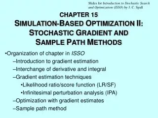
Slides for Introduction to Stochastic Search and Optimization ( ISSO ) by J. C. Spall. CHAPTER 15 S IMULATION - B ASED O PTIMIZATION II : S TOCHASTIC G RADIENT AND S AMPLE P ATH M ETHODS. Organization of chapter in ISSO Introduction to gradient estimation

CHAPTER 15 S IMULATION - B ASED O PTIMIZATION II : S TOCHASTIC G RADIENT AND S AMPLE P ATH M ETHODS
E N D
Presentation Transcript
Slides for Introduction to Stochastic Search and Optimization (ISSO)by J. C. Spall CHAPTER 15 SIMULATION-BASEDOPTIMIZATIONII: STOCHASTICGRADIENT AND SAMPLE PATHMETHODS Organization of chapter in ISSO Introduction to gradient estimation Interchange of derivative and integral Gradient estimation techniques Likelihood ratio/score function (LR/SF) Infinitesimal perturbation analysis (IPA) Optimization with gradient estimates Sample path method
Issues in Gradient Estimation • Estimate the gradient of the loss function with respect to parameters for optimization from simulation outputs where L(q) is a scalar-valued loss function to minimize and q is a p-dimensional vector of parameters • Essential properties of gradient estimates • Unbiased: • Small variance
Two Types of Parameters where V is the random effect in the system, is the probability density function of V • Distributional parametersqD: Elements of q that enter via their effect on probability distribution of V. For example, if scalar V has distribution N(m,s2), then m and s2 are distributional parameters • Structural parametersqS: Elements of q that have effects directly on the loss function (via Q) • Distinction not always obvious
Interchange of Derivative and Integral • Unbiased gradient estimations using only one simulation require the interchange of derivative and integral: • Above generally not true. Technical conditions needed for validity: • Q ·pV and are continuous • Above has implications in practical applications
A General Form of Gradient Estimate • Assume that all the conditions required for the exchange of derivative and integral are satisfied, • Hence, an unbiased gradient estimate can be obtained as Output from one simulation!
Two Gradient Estimates: LR/SF and IPA • Likelihood Ratio/ Score Function (LR/SF): only distributional parameters • Infinitestimal Perturbation Analysis (IPA): only structural parameters pure LR/SF pure IPA
Comparison of Pure LR/SF and IPA • In practice, neither extreme (LR/SF or IPA) may provide a framework for reasonable implementation: • LR/SF may require deriving a complex distribution function starting from U(0,1) • IPA may lead to intractable Q/qwith a complex Q(q,V) • Pure LR/SF gradient estimate tend to suffer from large variance (variance can grow with the number of components in V) • Pure IPA may result in a Q(q,V) that fails to meet the conditions for valid interchange of derivative and integral. Hence can lead to biased gradient estimate. • In many cases where IPA is feasible, it leads to low variance gradient estimate
A Simple Example: Exponential Distribution • Let Z be exponential random variable with mean q. That is . Define L = E(Z) =q. Then L/q = 1. • LR/SF estimate: V=Z; Q(q,V) =V. • IPA estimate: V=U(0,1); Q(q,V) = -qlogV (Z=-qlogV). • Both of LR/SF and IPA estimators are unbiased
Stochastic Optimization with Gradient Estimate • Use the gradient estimates in the root-finding stochastic approximation (SA) algorithm to minimize the loss function L(q) =E[Q(q,V)]: Find q* such that g(q*) =0 based on simulation outputs • A general root-finding SA algorithm: where ak is the step size with • If Yk is unbiased and has bounded variance (and other appropriate assumptions hold), then (a.s.) an estimate of
Simulation-Based Optimization • Use gradient estimate derived from one simulation run in the iteration of SA: where Vk is the realization of V from a simulation run with parameter q set at run one simulation with q= to obtain Vk derive gradient estimate from Vk iterate SA with the gradient estimate
Example: Experimental Response(Examples 15.4 and 15.5 in ISSO) • Let {Vk} be i.i.d. randomly generated binary (on-off) stimuli with “on” probability l. Assume Q(l,b,Vk) represents negative of specimen response, where b is design parameter. Objective is to design experiment to maximize the response (i.e., minimize Q) by selecting values for l and b. • Gradient estimate: q= [l, b]T; where and denotes derivative w.r.t. x
Experimental Response (continued) • Specific response function: where b is a structural parameter, but l is both a distributional and structural parameter. Then:
Sample Path Method • Sample path method based on reusing a fixed set of simulation runs • Method based on minimizing rather than L() • represents sample mean of N simulation runs • If N is large, then minimum of is close to minimum of L() (under conditions) • Optimization problem with is effectively deterministic • Can use standard nonlinear programming • IPA and/or LR/SF methods of gradient estimation still relevant • Generally need to choose a fixed value of (reference value) to produce the N simulation runs • Choice of reference value has impact on for finite N
Accuracy of Sample Path Method • Interested in accuracy of sample path method in seeking true optimal (minimum of L()) • Let represent minimum of surrogate loss • Let denote final solution from nonlinear programming method • Hence, error in estimate is due to two sources: • Error in nonlinear programming solution to finding • Difference in and • Triangle inequality can be used to provide bound to overall error: • Sometimes numerical values can be assigned to two right-hand terms in triangle inequality

