Download

1 / 64
650 likes | 812 Vues
Experimental design and statistical analyses of data. Lesson 4: Analysis of variance II A posteriori tests Model control How to choose the best model. Growth of bean plants in four different media. Completely randomized design (one-way anova). How to do it with SAS. DATA medium;

E N D
Experimental design and statistical analyses of data Lesson 4: Analysis of variance II A posteriori tests Model control How to choose the best model
Growth of bean plants in four different media Completely randomized design (one-way anova)
DATA medium; /* 20 bean plants exposed to 4 different treatments (5 plants per treatment) Mn = extra mangan added to the soil Zn = ekstra zink added to the soil Cu = ekstra cupper added to the soil K = control soil The dependent variable (Mass) is the biomass of the plants at harvest */ INPUT treat $ mass ; /* treat = treatment */ /* mass = biomass of a plant */ CARDS; zn 61.7 zn 59.4 zn 60.5 zn 59.2 zn 57.6 cu 57.0 cu 58.4 cu 57.3 cu 57.8 cu 59.9 mn 62.3 mn 66.2 mn 65.2 mn 63.7 mn 64.1 k 58.1 k 56.3 k 58.9 k 57.4 k 56.1 ;
PROC SORT;/* sort the observations according to treatment */ BY treat; RUN; /* compute average and 95% confidence limits for each treatment */ PROC MEANS N MEAN CLM; BY treat; RUN;
1 14:09 Wednesday, November 7, 2001 Analysis Variable : MASS ------------------------------------- TREAT=cu --------------------------------- N Mean Lower 95.0% CLM Upper 95.0% CLM -------------------------------------------------- 5 58.0800000 56.6550587 59.5049413 -------------------------------------------------- -------------------------------------- TREAT=k --------------------------------- N Mean Lower 95.0% CLM Upper 95.0% CLM -------------------------------------------------- 5 57.3600000 55.8866517 58.8333483 -------------------------------------------------- ------------------------------------- TREAT=mn --------------------------------- N Mean Lower 95.0% CLM Upper 95.0% CLM -------------------------------------------------- 5 64.3000000 62.4562230 66.1437770 -------------------------------------------------- ------------------------------------- TREAT=zn --------------------------------- N Mean Lower 95.0% CLM Upper 95.0% CLM -------------------------------------------------- 5 59.6800000 57.7777805 61.5822195 --------------------------------------------------
PROC GLM; CLASS treat; MODEL mass = treat /SOLUTION; /* SOLUTION gives the estimated parameter values */ RUN;
Class Levels Values TREAT 4 cu k mn zn Number of observations in data set = 20 General Linear Models Procedure Dependent Variable: MASS Sum of Mean Source DF Squares Square F Value Pr > F Model 3 145.82150 48.60717 26.72 0.0001 Error 16 29.10800 1.81925 Corrected Total 19 174.92950 R-Square C.V. Root MSE MASS Mean 0.833602 2.253439 1.3488 59.855 Source DF Type I SS Mean Square F Value Pr > F TREAT 3 145.82150 48.60717 26.72 0.0001 Source DF Type III SS Mean Square F Value Pr > F TREAT 3 145.82150 48.60717 26.72 0.0001
T for H0: Pr > |T| Std Error of Parameter Estimate Parameter=0 Estimate INTERCEPT 59.68000000 B 98.94 0.0001 0.60319980 TREAT cu -1.60000000 B -1.88 0.0791 0.85305334 k -2.32000000 B -2.72 0.0151 0.85305334 mn 4.62000000 B 5.42 0.0001 0.85305334 zn 0.00000000 B . . . NOTE: The X'X matrix has been found to be singular and a generalized inverse was used to solve the normal equations. Estimates followed by the letter 'B' are biased, and are not unique estimators of the parameters.
PROC GLM; CLASS treat; MODEL mass = treat /SOLUTION; /* SOLUTION gives the estimated parameter values */ /*Test for pairwise differences between treatmentsby linear contrasts */ CONTRAST 'Cu vs K' Treat 1 -1 0 0; CONTRAST 'Cu vs Mn' Treat 1 0 -1 0; CONTRAST 'Cu vs Zn' Treat 1 0 0 -1; CONTRAST 'K vs Mn' Treat 0 1 -1 0; CONTRAST 'K vs Zn' Treat 0 1 0 -1; CONTRAST 'Mn vs Zn' Treat 0 0 1 -1; /* test for whether the 3 treatments with added minerals aredifferent from the control */ CONTRAST 'K vs Cu, Mn Zn' Treat 1 -3 1 1; RUN;
Contrast DF Contrast SS Mean Square F Value Pr > F Cu vs K 1 1.29600 1.29600 0.71 0.4111 Cu vs Mn 1 96.72100 96.72100 53.17 0.0001 Cu vs Zn 1 6.40000 6.40000 3.52 0.0791 K vs Mn 1 120.40900 120.40900 66.19 0.0001 K vs Zn 1 13.45600 13.45600 7.40 0.0151 Mn vs Zn 1 53.36100 53.36100 29.33 0.0001 K vs Cu, Mn Zn 1 41.50017 41.50017 22.81 0.0002
PROC GLM; CLASS treat; MODEL mass = treat /SOLUTION; /* SOLUTION gives the estimated parameter values */ /* Test for differences between levels of treatment */ MEANS treat / BON DUNCAN SCHEFFE TUKEY DUNNETT('k'); RUN;
Tukey's Studentized Range (HSD) Test for variable: MASS NOTE: This test controls the type I experimentwise error rate. Alpha= 0.05 Confidence= 0.95 df= 16 MSE= 1.81925 Critical Value of Studentized Range= 4.046 Minimum Significant Difference= 2.4406 Comparisons significant at the 0.05 level are indicated by '***'. Simultaneous Simultaneous Lower Difference Upper TREAT Confidence Between Confidence Comparison Limit Means Limit mn - zn 2.1794 4.6200 7.0606 *** mn - cu 3.7794 6.2200 8.6606 *** mn - k 4.4994 6.9400 9.3806 *** zn - mn -7.0606 -4.6200 -2.1794 *** zn - cu -0.8406 1.6000 4.0406 zn - k -0.1206 2.3200 4.7606 cu - mn -8.6606 -6.2200 -3.7794 *** cu - zn -4.0406 -1.6000 0.8406 cu - k -1.7206 0.7200 3.1606 k - mn -9.3806 -6.9400 -4.4994 *** k - zn -4.7606 -2.3200 0.1206 k - cu -3.1606 -0.7200 1.7206
Bonferroni (Dunn) T tests for variable: MASS NOTE: This test controls the type I experimentwise error rate but generally has a higher type II error rate than Tukey's for all pairwise comparisons. Alpha= 0.05 Confidence= 0.95 df= 16 MSE= 1.81925 Critical Value of T= 3.00833 Minimum Significant Difference= 2.5663 Comparisons significant at the 0.05 level are indicated by '***'. Simultaneous Simultaneous Lower Difference Upper TREAT Confidence Between Confidence Comparison Limit Means Limit mn - zn 2.0537 4.6200 7.1863 *** mn - cu 3.6537 6.2200 8.7863 *** mn - k 4.3737 6.9400 9.5063 *** zn - mn -7.1863 -4.6200 -2.0537 *** zn - cu -0.9663 1.6000 4.1663 zn - k -0.2463 2.3200 4.8863 cu - mn -8.7863 -6.2200 -3.6537 *** cu - zn -4.1663 -1.6000 0.9663 cu - k -1.8463 0.7200 3.2863 k - mn -9.5063 -6.9400 -4.3737 *** k - zn -4.8863 -2.3200 0.2463 k - cu -3.2863 -0.7200 1.8463
Scheffe's test for variable: MASS NOTE: This test controls the type I experimentwise error rate but generally has a higher type II error rate than Tukey's for all pairwise comparisons. Alpha= 0.05 Confidence= 0.95 df= 16 MSE= 1.81925 Critical Value of F= 3.23887 Minimum Significant Difference= 2.6591 Comparisons significant at the 0.05 level are indicated by '***'. Simultaneous Simultaneous Lower Difference Upper TREAT Confidence Between Confidence Comparison Limit Means Limit mn - zn 1.9609 4.6200 7.2791 *** mn - cu 3.5609 6.2200 8.8791 *** mn - k 4.2809 6.9400 9.5991 *** zn - mn -7.2791 -4.6200 -1.9609 *** zn - cu -1.0591 1.6000 4.2591 zn - k -0.3391 2.3200 4.9791 cu - mn -8.8791 -6.2200 -3.5609 *** cu - zn -4.2591 -1.6000 1.0591 cu - k -1.9391 0.7200 3.3791 k - mn -9.5991 -6.9400 -4.2809 *** k - zn -4.9791 -2.3200 0.3391 k - cu -3.3791 -0.7200 1.9391
Dunnett's T tests for variable: MASS NOTE: This tests controls the type I experimentwise error for comparisons of all treatments against a control. Alpha= 0.05 Confidence= 0.95 df= 16 MSE= 1.81925 Critical Value of Dunnett's T= 2.592 Minimum Significant Difference= 2.2115 Comparisons significant at the 0.05 level are indicated by '***'. Simultaneous Simultaneous Lower Difference Upper TREAT Confidence Between Confidence Comparison Limit Means Limit mn - k 4.7285 6.9400 9.1515 *** zn - k 0.1085 2.3200 4.5315 *** cu - k -1.4915 0.7200 2.9315
Type I Tukey’s test is recommended as the best! Type II Duncan’s test exaggarates the risk of Type I errors Scheffe’s test exaggarates the risk of Type II errrors Comparison between multiple tests
PROC GLM; CLASS treat; MODEL mass = treat /SOLUTION; /* SOLUTION gives the estimated parameter values */ /* Test for differences between different levels of treatment */ MEANS treat / BON DUNCAN SCHEFFE TUKEY lines; RUN;
General Linear Models Procedure Duncan's Multiple Range Test for variable: MASS NOTE: This test controls the type I comparisonwise error rate, not the experimentwise error rate Alpha= 0.05 df= 16 MSE= 1.81925 Number of Means 2 3 4 Critical Range 1.808 1.896 1.951 Means with the same letter are not significantly different. Duncan Grouping Mean N TREAT A 64.3000 5 mn B 59.6800 5 zn B C B 58.0800 5 cu C C 57.3600 5 k
General Linear Models Procedure Tukey's Studentized Range (HSD) Test for variable: MASS NOTE: This test controls the type I experimentwise error rate, but generally has a higher type II error rate than REGWQ. Alpha= 0.05 df= 16 MSE= 1.81925 Critical Value of Studentized Range= 4.046 Minimum Significant Difference= 2.4406 Means with the same letter are not significantly different. Tukey Grouping Mean N TREAT A 64.3000 5 mn B 59.6800 5 zn B B 58.0800 5 cu B B 57.3600 5 k
General Linear Models Procedure Bonferroni (Dunn) T tests for variable: MASS NOTE: This test controls the type I experimentwise error rate, but generally has a higher type II error rate than REGWQ. Alpha= 0.05 df= 16 MSE= 1.81925 Critical Value of T= 3.01 Minimum Significant Difference= 2.5663 Means with the same letter are not significantly different. Bon Grouping Mean N TREAT A 64.3000 5 mn B 59.6800 5 zn B B 58.0800 5 cu B B 57.3600 5 k
General Linear Models Procedure Scheffe's test for variable: MASS NOTE: This test controls the type I experimentwise error rate but generally has a higher type II error rate than REGWF for all pairwise comparisons Alpha= 0.05 df= 16 MSE= 1.81925 Critical Value of F= 3.23887 Minimum Significant Difference= 2.6591 Means with the same letter are not significantly different. Scheffe Grouping Mean N TREAT A 64.3000 5 mn B 59.6800 5 zn B B 58.0800 5 cu B B 57.3600 5 k
PROC GLM; CLASS treat; MODEL mass = treat /SOLUTION; /* SOLUTION gives the estimated parameter values */ /* In unbalanced (and balanced) designs LSMEANS can be used: */ LSMEANS treat /TDIF PDIFF; RUN;
The GLM Procedure Least Squares Means LSMEAN treat mass LSMEAN Number cu 58.0800000 1 k 57.3600000 2 mn 64.3000000 3 zn 59.6800000 4 Least Squares Means for Effect treat t for H0: LSMean(i)=LSMean(j) / Pr > |t| Dependent Variable: mass i/j 1 2 3 4 1 0.844027 -7.29145 -1.87562 0.4111 <.0001 0.0791 2 -0.84403 -8.13548 -2.71964 0.4111 <.0001 0.0151 3 7.291455 8.135482 5.41584 <.0001 <.0001 <.0001 4 1.875615 2.719642 -5.41584 0.0791 0.0151 <.0001 NOTE: To ensure overall protection level, only probabilities associated with pre-planned comparisons should be used. Er denne P-værdi signifikant?
Signifikante P-værdier Den sekventielle Bonferroni-test Den sekventielle Bonferroni-test er mindre konservativ end den ordinære Bonferroni-test. Procedure: Først ordnes de k P-værdier i voksende rækkefølge. Lad P(i) betegne den i’te P-værdi efter at værdierne er blevet ordnet i voksende rækkefølge. Herefter beregnes hvor α er det signifikansniveau, der benyttes, hvis der kun var en enkelt P-værdi (sædvanligvis 0.05). Hvis P(i) < α(i) er den i’te P-værdi signifikant.
iid = independently and identically distributed Model assumptions and model control • All GLM’s are based on the assumption that (1) ε is independently distributed (2) ε is normally distributed with the mean = 0 (3) The variance of ε (denoted σ2) is the same for all values of the independent variable(s) (variance homogeneity) (4) Mathematically this is written as ε is iid ND(0; σ2)
Transformation of data • Transformation of data serves two purposes • To remove variance heteroscedasticity • To make data more normal Usually a transformation meets both purposes, but if this is not possible, variance homoscedasticity is regarded as the most important, especially if sample sizes are large
We have to find a value of p, so that the transformed values of y (denoted y*) y* = yp meet the condition of being normally distributed and with a variance that is independent of y*. A useful method to find p is to fit Taylor’s power law to data
Taylor’s power law It can be shown that p = 1- b/2 is the appropriate transformation we search for
If y is a proportion, i.e. 0 <= y <= 1, an appropriate transformation is often
T. urticae: log s2 = 1.303 + 1.943 log x r2 = 0.994 y* = log(y+1) P. persimilis: log s2 = 1.193 + 1.900 log x r2 = 0.992 y* = log(y+1)
b = birth rate/capita d = death rate/capita r = net growth rate/capita Instantaneous growth rate B = birth rate D = death rate N = population size at time t ΔN = change in N during Δt δ = noise associated with deaths ε = noise associated with births Exponential growth Deterministic model: Stochastic model: The number of births during a time interval follows a Poisson distribution with mean BΔt The probability that an individual dies during Δt is θ = DΔt/N The number of deaths during a time interval is binomially distributed with parameters (θ, N)
Type I, II, III and IV SS Example: Mites in stored grain influenced by temperature (T) and humidity (H)
DATA mites; INFILE'h:\lin-mod\besvar\opg1-1.prn' FIRSTOBS=2; INPUT pos $ depth T H Mites; /* pos = position in store */ /* depth = depth in m */ /* T = Temperature of grain */ /* H = Humidity of grain */ /* Mites = number of mites in sampling unit */ logMites = log10(Mites+1);/* log transformation of Mites */ T2 = T**2; /* square temperature */ H2 = H**2; /* square humidity */ TH = T*H; /* product of temperature and humidity */ PROC GLM; CLASS pos; MODEL logMites = T T2 H H2 TH /SOLUTION SS1 SS3; RUN;
General Linear Models Procedure Dependent Variable: LOGMITES Source DF Sum of Squares Mean Square F Value Pr > F Model 5 2.72839285 0.54567857 2.94 0.0265 Error 33 6.12429305 0.18558464 Corrected Total 38 8.85268590 R-Square C.V. Root MSE LOGMITES Mean 0.308199 85.66578 0.43079535 0.50287914 T for H0: Pr > |T| Std Error of Parameter Estimate Parameter=0 Estimate INTERCEPT 28.03994955 0.54 0.5902 51.56270293 T -0.86682324 -1.27 0.2147 0.68517409 T2 0.02333784 2.19 0.0358 0.01066368 H -3.52741058 -0.50 0.6235 7.11853025 H2 0.12548846 0.51 0.6161 0.24789107 TH 0.02315214 0.43 0.6702 0.05388643
General Linear Models Procedure Dependent Variable: LOGMITES Source DF Sum of Squares Mean Square F Value Pr > F Model 5 2.72839285 0.54567857 2.94 0.0265 Error 33 6.12429305 0.18558464 Corrected Total 38 8.85268590 R-Square C.V. Root MSE LOGMITES Mean 0.308199 85.66578 0.43079535 0.50287914 Source DF Type I SS Mean Square F Value Pr > F T 1 0.22115656 0.22115656 1.19 0.2829 T2 1 1.38171889 1.38171889 7.45 0.0101 H 1 1.03546840 1.03546840 5.58 0.0242 H2 1 0.05579073 0.05579073 0.30 0.5872 TH 1 0.03425827 0.03425827 0.18 0.6702 Source DF Type III SS Mean Square F Value Pr > F T 1 0.29703065 0.29703065 1.60 0.2147 T2 1 0.88889243 0.88889243 4.79 0.0358 H 1 0.04556941 0.04556941 0.25 0.6235 H2 1 0.04755847 0.04755847 0.26 0.6161 TH 1 0.03425827 0.03425827 0.18 0.6702
Example: β3 SS I is used to compare the model: with SS III is used to compare the model with
General Linear Models Procedure Dependent Variable: LOGMITES Source DF Sum of Squares Mean Square F Value Pr > F Model 5 2.72839285 0.54567857 2.94 0.0265 Error 33 6.12429305 0.18558464 Corrected Total 38 8.85268590 R-Square C.V. Root MSE LOGMITES Mean 0.308199 85.66578 0.43079535 0.50287914 Source DF Type I SS Mean Square F Value Pr > F T 1 0.22115656 0.22115656 1.19 0.2829 T2 1 1.38171889 1.38171889 7.45 0.0101 H 1 1.03546840 1.03546840 5.58 0.0242 H2 1 0.05579073 0.05579073 0.30 0.5872 TH 1 0.03425827 0.03425827 0.18 0.6702 Source DF Type III SS Mean Square F Value Pr > F T 1 0.29703065 0.29703065 1.60 0.2147 T2 1 0.88889243 0.88889243 4.79 0.0358 H 1 0.04556941 0.04556941 0.25 0.6235 H2 1 0.04755847 0.04755847 0.26 0.6161 TH 1 0.03425827 0.03425827 0.18 0.6702 H is significant if it is added after T and T2 H is not significant if it is added after T, T2, H2, and TH
DATA mites; INFILE'h:\lin-mod\besvar\opg1-1.prn' FIRSTOBS=2; INPUT pos $ depth T H Mites; /* pos = position in store */ /* depth = depth in m */ /* T = Temperature of grain */ /* H = Humidity of grain */ /* Mites = number of mites in sampling unit */ logMites = log10(Mites+1);/* log transformation of Mites */ T2 = T**2; /* square temperature */ H2 = H**2; /* square humidity */ TH = T*H; /* product of temperature and humidity */ PROC STEPWISE; MODEL logMites = T T2 H H2 TH /MAXR; RUN;
Maximum R-square Improvement for Dependent Variable LOGMITES Step 1 Variable H2 Entered R-square = 0.11939020 C(p) = 7.00650467 DF Sum of Squares Mean Square F Prob>F Regression 1 1.05692394 1.05692394 5.020.0312 Error 37 7.79576196 0.21069627 Total 38 8.85268590 Parameter Standard Type II Variable Estimate Error Sum of Squares F Prob>F INTERCEP -2.00838948 1.12364950 0.67311767 3.19 0.0821 H2 0.01218833 0.00544190 1.05692394 5.02 0.0312 Bounds on condition number: 1, 1 ----------------------------------------------------------------------------------- The above model is the best 1-variable model found.
Step 2 Variable T Entered R-square = 0.14111324 C(p) = 7.97028096 DF Sum of Squares Mean Square F Prob>F Regression 2 1.24923115 0.62461557 2.960.0647 Error 36 7.60345475 0.21120708 Total 38 8.85268590 Parameter Standard Type II Variable Estimate Error Sum of Squares F Prob>F INTERCEP -1.75010488 1.15711557 0.48315129 2.29 0.1391 T -0.02071757 0.02171178 0.19230720 0.91 0.3463 H2 0.01202664 0.00545113 1.02807459 4.87 0.0338 Bounds on condition number: 1.000967, 4.003869
Step 3 Variable H2 Removed R-square = 0.18352305 C(p) = 5.94726448 Variable TH Entered DF Sum of Squares Mean Square F Prob>F Regression 2 1.62467193 0.81233596 4.05 0.0260 Error 36 7.22801397 0.20077817 Total 38 8.85268590 Parameter Standard Type II Variable Estimate Error Sum of Squares F Prob>F INTERCEP 0.72634839 0.24079746 1.82684898 9.10 0.0047 T -0.52367627 0.19084468 1.51175757 7.53 0.0094 TH 0.03507940 0.01326789 1.40351537 6.99 0.0121 Bounds on condition number: 81.35444, 325.4178 The above model is the best 2-variable model found.
Step 4 Variable T2 Entered R-square = 0.30260874 C(p) = 2.26668560 DF Sum of Squares Mean Square F Prob>F Regression 3 2.67890010 0.89296670 5.06 0.0051 Error 35 6.17378580 0.17639388 Total 38 8.85268590 Parameter Standard Type II Variable Estimate Error Sum of Squares F Prob>F INTERCEP 3.12310821 1.00603496 1.69993153 9.64 0.0038 T -0.94651154 0.24882419 2.55240831 14.47 0.0005 T2 0.02187819 0.00894923 1.05422818 5.98 0.0197 TH 0.03099168 0.01254804 1.07602465 6.10 0.0185 Bounds on condition number: 157.4125, 1019.366 ----------------------------------------------------------------------------------- The above model is the best 3-variable model found.
Step 5 Variable H2 Entered R-square = 0.30305192 C(p) = 4.24554515 DF Sum of Squares Mean Square F Prob>F Regression 4 2.68282344 0.67070586 3.70 0.0133 Error 34 6.16986246 0.18146654 Total 38 8.85268590 Parameter Standard Type II Variable Estimate Error Sum of Squares F Prob>F INTERCEP 2.56528922 3.92853717 0.07737622 0.43 0.5182 T -0.85413336 0.67705608 0.28880097 1.59 0.2157 T2 0.02264025 0.01045241 0.85138509 4.69 0.0374 H2 0.00311049 0.02115432 0.00392334 0.02 0.8840 TH 0.02338380 0.05328321 0.03494992 0.19 0.6635 Bounds on condition number: 1451.704, 10936.61
Step 6 Variable TH Removed R-square = 0.30432962 C(p) = 4.18459648 Variable H Entered DF Sum of Squares Mean Square F Prob>F Regression 4 2.69413458 0.67353364 3.72 0.0129 Error 34 6.15855132 0.18113386 Total 38 8.85268590 Parameter Standard Type II Variable Estimate Error Sum of Squares F Prob>F INTERCEP 26.64541542 50.83962556 0.04975537 0.27 0.6036 T -0.58573429 0.20112070 1.53634027 8.48 0.0063 T2 0.02565523 0.00908804 1.44347920 7.97 0.0079 H -3.55394542 7.03238763 0.04626106 0.26 0.6166 H2 0.13533410 0.24385185 0.05579073 0.31 0.5825 Bounds on condition number: 2335.775, 19486.21 ----------------------------------------------------------------------------------- The above model is the best 4-variable model found.
Step 7 Variable TH Entered R-square = 0.30819944 C(p) = 6.00000000 DF Sum of Squares Mean Square F Prob>F Regression 5 2.72839285 0.54567857 2.94 0.0265 Error 33 6.12429305 0.18558464 Total 38 8.85268590 Parameter Standard Type II Variable Estimate Error Sum of Squares F Prob>F INTERCEP 28.03994954 51.56270293 0.05488139 0.30 0.5902 T -0.86682324 0.68517409 0.29703065 1.60 0.2147 T2 0.02333784 0.01066368 0.88889243 4.79 0.0358 H -3.52741058 7.11853025 0.04556941 0.25 0.6235 H2 0.12548846 0.24789107 0.04755847 0.26 0.6161 TH 0.02315214 0.05388643 0.03425827 0.18 0.6702 Bounds on condition number: 2355.783, 37061.88 ----------------------------------------------------------------------------------- The above model is the best 5-variable model found. No further improvement in R-square is possible.