Go over: Geometric correction
Go over: Geometric correction. Selection of GCPS; Coor transform; DN Resampling. Registration or Rectification. Rotate Scale Transform. How to remove noise from an image? How to highlight edges within the image?. Spatial-based Enhancements. Lecture 5 prepared by R. Lathrop 10/99

Go over: Geometric correction
E N D
Presentation Transcript
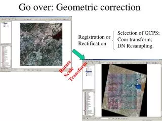
Go over: Geometric correction Selection of GCPS; Coor transform; DN Resampling. Registration or Rectification Rotate Scale Transform
How to remove noise from an image? How to highlight edges within the image?
Spatial-based Enhancements Lecture 5 prepared by R. Lathrop 10/99 updated 2/05 ERDAS Field Guide 5th Ed. Ch 5:154-162
Main points of the lecture • Concept of spatial frequency • Texture • Low vs. Hi frequency enhancement: kernel convolution. • Edge Enhancement/Sharpening • Edge Detection/Extraction • Global vs. local operator: Fourier vs. kernel convolution
Spatial frequency • Spatial frequency is the number of changes in brightness value per unit distance in any part of an image • low frequency - tonally smooth, gradual changes • high frequency - tonally rough, abrupt changes
Spatial Frequencies Zero Spatial frequency Low Spatial frequency High Spatial frequency Example from ERDAS IMAGINE Field Guide, 5th ed.
Spatial vs. Spectral Enhancement • Spatial-based Enhancement modifies a pixel’s values based on the values of the surrounding pixels (local operator) • Spectral-based Enhancement modifies a pixel’s values based solely on the pixel’s values (point operator)
Moving Window concept Kernel scans across row, then down a row and across again, and so on.
Focal Analysis • Mathematical calculation of pixel DN values within moving window • Mean, Median, Std Dev., Majority • Focal value written to center pixel in moving window
Noise Removal • Noise: extraneous unwanted signal response • SNR measures the radiometric accuracy of the data. Want high Signal-to-noise-ratio (SNR) • Over low reflectance targets (i.e. dark pixels such as clear water) the noise may swamp the actual signal True Signal Observed Signal Noise +
Noise Removal • Noise removal techniques to restore image to as close an approximation of the original scene as possible • Bit errors: random pixel to pixel variations, average neighborhood (e.g., 3x3) using a moving window (convolution kernel) • Destriping: correct defective sensor • Line drop: average lines above and below
Example: Line drop • 105 156 178 154 167 200 202 205 • ----- ----- ---- ----- ----- ----- ----- ----- • 107 152 166 165 173 204 204 207 • Interpolated: above and below to fill line • 156 178 154 167 200 202 205 • 106 154 172 160 170 202 203 206 • 107 152 166 165 173 204 204 207
Texture • Texture: variation in BV’s in a local region, gives estimate of local variability. Can be used as another layer of data in classification/ interpretation process. • 1st order statistics: mean Euclidean distance • 2nd order: range, variance, std dev • 3rd order: skewness • 4th order: kurtosis • Window size will affect results. Often need larger moving window sizes for proper enhancement.
Example Image: Ikonos pan Orignal IKONOS pan
Texture: variance 3x3 texture 7x7 texture
Statistical or Sigma Filters: often used for radar imagery enhancement • Center pixel is replaced by the average of all pixel values within the moving window that fall within the designated range of sigma: µ+σ • Sigma may represent the coefficient of variation. The default sigma value (set to 0.15 in ERDAS IMAGINE) can be modified using multipliers to increase or decrease the range of values within the moving window used to calculate the average. • Use the filter sequentially with increasing multipliers to preserve fine detail while smoothing the image.
Spatial-based Enhancement • Low vs. Hi frequency enhancement • Edge Enhancement/Sharpening • Edge Detection/Extraction • Many spatial-based enhancement (filtering) techniques use kernel convolution, a type of local operation
Example: kernel convolution 8 8 6 6 6 2 8 6 6 6 2 2 8 6 6 2 2 2 8 6 2 2 2 2 8 -1 -1 -1 -1 16 -1 -1 -1 -1 Convolution Kernel Example from ERDAS IMAGINE Field Guide, 5th ed.
Pixel Convolution Where i = row location, j = column location fij = the coefficient of a convolution kernel at position i, j dij = the BV of the original data at position i, j q = the dimension of the kernel, assuming a square kernel , i.e., either the sum of the coefficients of the kernel or 1 if the sum of coefficients is zero BV = output pixel value
Example: kernel convolution Original: 8 6 6 2 8 6 2 2 8 Kernel: -1 -1 -1 -1 16 -1 -1 -1 -1 Result = 11 X J=1 j=2 j=3 I=1 (-1)(8) + (-1)(6) + (-1)(6) = -8 -6 -6 = -20 I=2 (-1)(2) + (16)(8) + (-1)(6) = -2 +128 -6 = 120 I=3 (-1)(2) + (-1)(2) + (-1)(8) = -2 -2 -8 = -12 F = 16 - 8 = 8 Sum = 88 output BV = 88 / 8 = 11
Example: kernel convolution Input Output 8 6 6 6 6 2 8 6 6 6 2 2 8 6 6 2 2 2 8 6 2 2 2 2 8 11 6 6 6 6 0 11 6 6 6 2 0 11 6 6 2 2 0 11 6 2 2 2 0 11 Edge
Low vs. high spatial frequency enhancements • Low frequency enhancers (low pass filters): Emphasize general trends, smooth image • High frequency enhancers (high pass filters): Emphasize local detail, highlight edges
Example: Low Frequency Enhancement Kernel: 1 1 1 1 1 1 1 1 1 Low value surrounded by higher values Original: 204 200 197 201 100 209 198 200 210 Output: 204 200 197 201 191 209 198 200 210 High value surrounded by lower values Original: 64 60 57 61 125 69 58 60 70 Output: 64 60 57 61 65 69 58 60 70 From ERDAS Field Guide p.111
Low pass filter Orignal IKONOS pan 7x7 low pass
Gaussian filter • Gaussian smoothing filter is similar to a low pass mean filter but uses a kernel that represents the shape of a Gaussian (“bell-shaped”) curve. • Example Graphic taken from http://homepages.inf.ed.ac.uk/rbf/HIPR2/gsmooth.htm
Example: High Frequency Enhancement Kernel: -1 -1 -1 -1 16 -1 -1 -1 -1 Low value surrounded by higher values Original: 204 200 197 201 120 209 198 200 199 Output: 204 200 197 201 39 209 198 200 210 High value surrounded by lower values Original: 64 50 57 61 125 69 58 60 70 Output: 64 50 57 61 187 69 58 60 70 From ERDAS Field Guide p.111
High Pass filter -1 -1 -1 -1 9 -1 -1 -1 -1 -1 -1 -1 -1 17 -1 -1 -1 -1 3x3 high pass 3x3 edge enhance
Edge detection • Edge detection process: Smooth out areas of low spatial frequency and highlight edges (i.e., local changes between bright vs. dark features) • Zero-sum kernels: - linear edge/line detecting templates - directional (compass templates) - non-directional (Laplacian)
Zero sum kernels • Zero sum kernels: the sum of all coefficients in the kernel equals zero. In this case, F is set = 1 since division by zero is impossible • zero in areas where all input values are equal • low in areas of low spatial frequency • extreme in areas of high spatial frequency (high values become higher, low values lower)
Example: Linear Edge Detecting Templates Vertical: -1 0 1 Horizontal: -1 -1 -1 -1 0 1 0 0 0 -1 0 1 1 1 1 Diagonal Diagonal (NW-SE): 0 1 1 (NE-SW): 1 1 0 -1 0 1 1 0 -1 -1 -1 0 0 -1 -1 Example: vertical template convolution Original: 2 2 2 8 8 8 Output: 0 18 18 0 0 2 2 2 8 8 8 0 18 18 0 0 2 2 2 8 8 8 0 18 18 0 0
Linear Edge Detection -1 -2 -1 0 0 0 1 2 1 -1 0 1 -2 0 2 -1 0 1 Horizontal Edge Vertical Edge
Linear Line Detecting Templates • Narrow (single pixel wide) line features (i.e. rivers and roads) are output as pairs of edges using linear edge detection templates. To create a single line edge feature, a linear line detecting template can be used Vertical: -1 2 -1 Horizontal: -1 -1 -1 -1 2 -1 2 2 2 -1 2 -1 -1 -1 -1
Example: Linear Line Detecting Templates Vertical: -1 2 -1 Horizontal: -1 -1 -1 -1 2 -1 2 2 2 -1 2 -1 -1 -1 -1
Linear Line Detection -1 -1 -1 2 2 2 -1 -1 -1 -1 2 -1 -1 2 -1 -1 2 -1 Horizontal Edge Vertical Edge
Compass gradient masks Produce a maximum output for vertical (or horizontal) brightness value changes from the specified direction. For example a North compass gradient mask enhances changes that increase in a northerly direction, i.e. from south to north: North: 1 1 1 1 -2 1 -1 -1 -1
Example: Compass gradient masks North: 1 1 1 South: -1 -1 -1 1 -2 1 1 -2 1 -1 -1 -1 1 1 1 Example: North vs. south gradient mask North South Original: 8 8 8 Output: . . . Output: . . . 8 8 8 0 0 0 0 0 0 8 8 8 18 18 18 -18 -18 -18 2 2 2 18 18 18 -18 -18 -18 2 2 2 0 0 0 0 0 0 2 2 2 . . . . . .
Directional gradient filters • Directional gradient filters produce output images whose BVs are proportional to the difference between neighboring pixel BVs in a given direction, i.e. they calculate the directional gradient • Spatial differencing: calculating spatial derivatives (differencing a pixel from its neighbor or some other lag distance); doesn’t use kernel convolution approach • Vertical: BVi,j = BVi,j - BVi,j+1 + K • Horizontal: BVi,j = BVi,j - BVi-1,j + K constant K added to make output positive (usually K=127)
Directional gradient filters Example: horizontal spatial difference BVi,j = BVi,j - BVi-1,j + K Original: 2 2 2 8 8 8 Output: 0 0 6 0 0 2 2 2 8 8 8 0 0 6 0 0 8 8 8 2 2 2 0 0 -6 0 0 8 8 8 2 2 2 0 0 -6 0 0 Positive values signify increase left to right Negative values signify decrease left to right
Non-directional Edge Enhancement • Laplacian is a second derivative and is insensitive to direction. Laplacian highlights points, lines and edges in the image and suppresses uniform, smoothly varying regions • 0 -1 0 1 -2 1 -1 4 -1 -2 4 -2 0 -1 0 1 -2 1
Nonlinear Edge Detection Sobel edge detector: a nonlinear combination of pixels Sobel = SQRT(X2 + Y2) X: -1 0 1 Y: 1 2 1 -2 0 2 0 0 0 -1 0 1 -1 -2 -1
Nondirectional edge filter Laplacian filter Sobel filter
Edge Enhancement • Edge enhancement process: • First detect/map the edges • Add or subtract the edges back into the original image to increase contrast in the vicinity of the edge
Original – edge = edge enhanced Original IKONOS pan - Edge enhancement Laplacian
Unsharp masking to enhance detail Original IKONOS pan - Original – low pass = edge enhanced 7x7 low
High Pass Filter (HPF) method for Image Fusion • Capture high frequency information from the high spatial resolution panchromatic image using some form of high pass filter • This high frequency information then added into the low spatial resolution multi-spectral imagery • Often produces less distortion to the original spectral characteristics of the imagery but also less visually attractive
Edge Mapping/Extraction • BV thresholding of the edge detector output to create a binary map of edges vs. non-edges • Threshold too low: too many isolated pixels classified as edges and edge boundaries too thick • Threshold too high: boundaries will consist of thin, broken segments
Edge Mapping/Extraction:example using Sobel filter Edge image represents a continuous range of values. Can you determine a threshold? +
Edge Mapping/Extraction:example using Sobel filter Edge-extracted image DN = 15 Edge-extracted image DN = 20
Adaptive Filtering • The selection of a single threshold to differentiate an edge that is applicable across the entire image may be difficult • An adaptive filtering approach that looks at the relative difference on a more local scale (i.e., within a moving window) may achieve better results.