Download
1 / 15
200 likes | 588 Vues
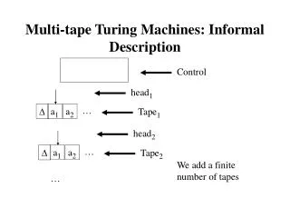
Control. head 1. head 2. …. …. a 1. a 1. a 2. a 2. . . Tape 1. Tape 2. Multi-tape Turing Machines: Informal Description. We add a finite number of tapes. …. ( (p,( x 1 , x 2 )), (q, ( y 1 , y 2 )) ). Such that each x i is in and each y i is in or is or .

E N D
Control head1 head2 … … a1 a1 a2 a2 Tape1 Tape2 Multi-tape Turing Machines: Informal Description We add a finite number of tapes …
( (p,(x1, x2)), (q, (y1, y2)) ) Such that each xi is in and each yi is in or is or . and if xi = then yi = or yi = Multi-tape Turing Machines: Informal Description (II) • Each tape is bounded to the left by a cell containing the symbol • Each tape has a unique header • Transitions have the form (for a 2-tape Turing machine):
Input: Tape1: w Tape2: Output: Tape1: 1… if w L or Tape1: 0… if w L Multi-tape Turing Machines Construct a 2-tape Turing machine that recognizes the language: L = {anbn : n = 0, 1, 2, …} • Hints: • use the second tape as an stack • Use the machines M1 and M0
Multi-tape Turing Machines vs Turing Machines M2 … a1 a2 ai … … … b1 b2 bj • We can simulate a 2-tape Turing machine M2 in a Turing machine M: • we can represent the contents of the 2 tapes in the single tape by using special symbols • We can simulate one transition from the M2 by constructing multiple transitions on M • We introduce several (finite) new states into M
State in the Turing machine M: “s+b+1+a+2” Which represents: Using States to “Remember” Information Configuration in a 2-tape Turing Machine M2: Tape1 a b a b State: s Tape2 b b a • M2 is in state s • Cell pointed by first header in M2 contains b • Cell pointed by second header in M2 contains an a
(# states in M2) * | or or | * | or or | State in the Turing machine M: “s+b+1+a+2” Using States to “Remember” Information (2) How many states are there in M? Yes, we need large number of states for M but it is finite!
4 e a b 3 b b 1 2 a b a Configuration in a 2-tape Turing Machine M2: Tape1 a b a b State in M2: s Tape2 b b a Equivalent configuration in a Turing Machine M: State in M: s+b+1+a+2
Simulating M2 with M • The alphabet of the Turing machine M extends the alphabet 2 from the M2 by adding the separator symbols: 1, 2, 3 , 4 and e, and adding the mark symbols: and • We introduce more states for M, one for each 5-tuple p++1+ +2where p in an state in M2 and +1+ +2indicates that the head of the first tape points to and the second one to • We also need states of the form p++1++2 for control purposes
At the beginning of each iteration of M2, the head starts at e and both M and M2 are in an state s • We traverse the whole tape do determine the state p++1+ +2,Thus, the transition in M2 that is applicable must have the form: State in M: s+b+1+a+2 4 e a b 3 b b 1 2 a b a ( (p,(, )), (q,(,)) ) in M2 p+ +1+ +2 q+ +1++2 in M Simulating transitions in M2 with M
i i 1 … 1 … Simulating transitions in M2 with M (2) • To apply the transformation (q,(,)),we go forwards from the first cell. • If the (or ) is (or ) we move the marker to the right (left): • If the (or ) is a character, we first determine the correct position and then overwrite
Output: 4 e a b 3 b b 2 1 a b a 4 e 1 a b 3 b b 2 a b a 4 e 3 b b a a 1 b 2 a b 4 e 1 3 b b 2 a b a b a 4 e a b 3 b b 2 1 a b a state: s 4 e a b 3 b b 2 1 a b a state: s+b+1
Multi-tape Turing Machines vs Turing Machines (6) • We conclude that 2-tape Turing machines can be simulated by Turing machines. Thus, they don’t add computational power! • Using a similar construction we can show that 3-tape Turing machines can be simulated by 2-tape Turing machines (and thus, by Turing machines). • Thus, k-tape Turing machines can be simulated by Turing machines
Implications • If we show that a function can be computed by a k-tape Turing machine, then the function is Turing-computable • In particular, if a language can be decided by a k-tape Turing machine, then the language is decidable Example: Since we constructed a 2-tape TM that decides L = {anbn : n = 0, 1, 2, …}, then L is Turing-computable.
Implications (2) Example: Show that if L1 and L2 are decidable then L1 L2 is also decidable Proof. …
Homework • Prove that (ab)* is Turing-enumerable (Hint: use a 2-tape Turing machine.) • Exercise 4.24 a) and b) (Hint: use a 3-tape Turing machine.) • For proving that * is Turing-enumerable, we needed to construct a Turing machine that computes the successor of a word. Here are some examples of what the machine will produce (w w’ indicates that when the machine receives w as input, it produces w’ as output) • a b aa ab ba bb aaa