Nuclear Model Codes at Yale Computer name: Titan
Addendum to IBA slides to aid in practical calculations See slides 4,5 (Slides 2,3 6,7 below are essentially repeated from Lecture 3 so that this Addendum is self-contained). Nuclear Model Codes at Yale Computer name: Titan. Connecting to SSH: Quick connect

Nuclear Model Codes at Yale Computer name: Titan
E N D
Presentation Transcript
Addendum to IBA slides to aid in practical calculations See slides 4,5 (Slides 2,3 6,7 below are essentially repeated from Lecture 3 so that this Addendum is self-contained)
Nuclear Model Codes at YaleComputer name: Titan Connecting to SSH: Quick connect Host name: titan.physics.yale.edu User name: phy664 Port Number 22 Password: nuclear_codes cd phintm pico filename.in (ctrl x, yes, return) runphintm filename (w/o extension) pico filename.out (ctrl x, return)
c Mapping the Entire Triangle with a minimum of data H =ε nd - Q Q Parameters: , c (within Q) /ε /εvaries from 0 to infinity 2 parameters 2-D surface /ε Note: The natural size of QQ is much larger than ndso, in typical fits, is on the order of 10’s of keV andε is ~ hundreds of keV Note: we usually keep fixed at 0.02 MeV and just vary ε. When we have a good fit to RELATIVE energies, we then scale BOTH and ε by the same factor to reproduce the experimental scale of energies
One awkward thing about IBA calculations in the triangle and its solution – an infinity /ε varies from zero at U(5) to infinity along the SU(3) — O(6) line. That is a large range to span !! Better to re-write the Hamiltonian in terms of another parameter with range 0 – 1.
0+ 4+ 2+ 2.5 1 2+ 0 0+ ζ H = c [ ( 1 – ζ ) nd - O(6) Qχ ·Qχ ] ζ = 1, χ = 0 4NB 2γ+ χ 0+ 4+ 2+ 0+ 4+ 2.0 3.33 1 2+ 2+ 1 ζ 0 0+ 0+ 0 U(5) SU(3) ζ = 0 ζ = 1, χ = -1.32 Now ζ varies from 0 – 1and its value is simply proportional to the distance from U(5) to the far side of the triangle Usual procedure: Set = 0.02, fitζ, then re-scale both and ε to match level scheme. Note that the contours in the triangle are BOSON NUMBER-dependent
H has two parameters. A given observable can only specify one of them. That is, a given observable has a contour (locus) of constant values in the triangle R4/2 = 2.9 Structure varies considerably along this trajectory, so we need a second observable.
Mapping Structure with Simple Observables – Technique of Orthogonal Crossing Contours γ - soft Vibrator Rotor Note that these contours depend on boson number so they have to be constructed for each boson number (although, to a good approximation, a given set can be used for adjacent boson numbers as well) R. BurcuCakirli McCutchan and Zamfir