Pole Placement Design Approaches in Polynomial Control Systems
Explore the algebraic problem of finding polynomials R(z) and S(z) satisfying specific conditions in controller design. Learn about Diophantine Equation, Regulator Design, and Pole Placement for optimal system control.

Pole Placement Design Approaches in Polynomial Control Systems
E N D
Presentation Transcript
I/O Model where and are polynomials in forward-shift operator q. Basic assumptions i) deg B(q) < deg A(q) ii) A(q) and B(q) do not have any common factors. (coprime) iii) The polynomial of A(q) is monic. (normalized for uniqueness) Note: Pulse transfer function B(z)/A(z)
Controller where R(q), T(q)and S(q) are polynomials in forward-shift operator. R(q) can be chosen so that the coefficient of the term of the highest power in q is unity. Notes: deg R(z) deg T(z) deg R(z) deg S(z) causal controller
The characteristic polynomial of the closed-loop system if there is a time delay in the control law of one sampling period
Pole Placement Design Algebraic problem of finding polynomials R(z) and S(z) that satisfy (4) for given A(z), B(z) and Acl(z)
It is natural to choose the polynomial T(z) so that it cancels the observer polynomial Ao(z). where to is the desired static gain of the system.
Diophantine Equation Let A, B, and C be polynomials with real coefficients and X and Y unknown polynomials. Then the above equation has a solution iff the greatest common factor of A and B divides C. Notes: i) The Diophantine equation has many other names in literature, the Bezout identity or the Aryabhatta’s identity. ii) iii) The extended Euclidean algorithm is a straightforward method to solve the Diophantine equation.
Regulator Design by Pole Placement - polynomial equation approach
Pulse transfer function(uc to y) Remarks: • Causality • deg R deg T • deg R deg S • deg A deg B • Uniqueness • deg A > deg S, deg B > deg R • iii) The cancelled factors must correspond to stable modes.
Minimum Variance Control - system with stable inverse