Additional Aspects of Aqueous Equilibria

1. Additional Aspects of Aqueous Equilibria BLB 11th Chapter 17

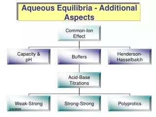
2. Buffered Solutions (sections 1-2) Acid/Base Reactions & Titration Curves (3) Solubility Equilibria (sections 4-5) Two important points: • Reactions with strong acids or strong bases go to completion. • Reactions with only weak acids and bases reach an equilibrium.

3. 17.1 The Common Ion Effect • What affect does the addition of its conjugate base have on the weak acid equilibrium? On the pH? Used in making buffered solutions

4. Calculate the pH of a 0.60 M HF solution. The Ka of HF is 7.2×10-4.

5. Calculate the pH of a solution containing 0.60 M HF and 1.00 M KF.

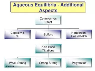
6. 17.2 Buffered Solutions • Resist a change in pH upon the addition of small amounts of strong acid or strong base • Consist of a weak conjugate acid-base pair • Control pH at a desired level (pKa) • Examples: blood (p. 729), physiological fluids, seawater, foods

7. How do buffers work?

8. Calculating pH of a Buffer Henderson-Hasselbalch equation

9. Calculate the pH of a solution containing 0.60 M HF and 1.00 M KF. (again, but the easy way)

10. Adding strong acid or base to a buffer Adding acid: H3O+ + HA or A- → Adding base: OH- + HA or A-→ Calculating pH: • Stoichiometry of added acid or base • Equilibrium problem (H-H equation)

11. Calculate the pH after adding 0.20 mol of HCl to 1.0 L of the 0.60 M HF and 1.00 M KF buffer.

12. Calculate the pH after adding 0.10 mol of NaOH to 1.0 L of the 0.60 M HF and 1.00 M KF buffer.

13. Calculate the pH for a 1.0-L solution that contains 0.25 M NH3 and 0.15 M NH4Br. Kb=1.8x10-5 for NH3

14. Calculate the pH for a 1.0-L solution that contains 0.25 M NH3 and 0.15 M NH4Br after the addition of 0.05 mol of RbOH.

15. Calculate the pH for a 1.0-L solution that contains 0.25 M NH3 and 0.15 M NH4Br after the addition of 0.35 mol of HCl.

16. Buffers (wrap up) • H-H equation • No 5% check • When strong acid or base is added, start reaction with that acid or base. • Making buffers of a specific pH? H-H equation • Buffer capacity exceeded – when added acid or base totally consumes a buffer component (p. 726)

17. How would you prepare a phenol buffer to control pH at 9.50? Ka = 1.3x10-10 for phenol

18. 17.3 Acid-Base Titrations • Titration – a reaction used to determine concentration (acid-base, redox, precipitation) • Titrant – solution in buret; usually a strong base or acid • Analyte – solution being titrated; often the unknown • @ equivalence point (or stoichiometric point): mol acid = mol base • Found by titration with an indicator • Solution not necessarily neutral • pH dependent upon salt formed • pH titration curve – plot of pH vs. titrant volume

19. Acid-base Titration Reactions and Curves • Recognize curve types • Calculate pH at various points on curve.

20. Type 1: Strong acid + strong base • Goes to completion • Forms a neutral salt • Equivalence point - neutral solution, [H3O+] = 1.0 x 10-7 M, pH = 7.00 • pH calculations involve only stoichiometry and excess H3O+ and OH-

21. Strong acid – Strong base

22. Type 1: Strong acid + strong base20.0 mL 0.200 M HClO4 titrated with 0.200 M KOH Initial mmol acid =

23. Another SA/SB titration10.0 mL 0.20 M KOH titrated with 0.10 M HCl Initial mmol base =

24. Type 2: Weak acid + strong base • Titration reaction goes to completion • Forms a basic salt (from conj. base of the weak acid) • Equivalence point - basic solution, pH > 7.00 • pH calculations involve stoichiometry and equilibrium

25. Weak acid – Strong base

26. Type 2: Weak acid + strong base25.0 mL 0.100M HC3H5O2 titrated with 0.100 M KOHKa = 1.3x10-5 Calculate the pH at the following points: • Initial (0.00 mL KOH) • 10.00 mL KOH • Midpoint (12.50 mL KOH) • Equivalence pt. (25.00 mL KOH) • 10.00 mL after eq. pt. (35.00 mL KOH)

27. Polyprotic Weak acid – Strong base

28. Type 3: Weak base + strong acid • Titration reaction goes to completion • Forms an acidic salt (from conj. acid of the weak base) • Equivalence point - acidic solution, pH < 7.00 • pH calculations involve stoichiometry and equilibrium

29. Strong base – Strong acid Weak base – Strong acid Strong base Weak base

30. Type 3: Weak base + strong acid 25.0 mL 0.150 M NH3 titrated with 0.100 M HCl Kb = 1.8x10-5 Calculate the pH at the following points: • Initial (0.00 mL HCl) • Midpoint (______ mL HCl) • 25.00 mL HCl • Equivalence pt. (______ mL HCl) • 10.00 mL after eq. pt. (______ mL HCl)

31. Types 2 & 3 pH Calculations • Initial pH – same as weak acid or base problem (chapter 16) • Before equivalence point – Buffer • @ midpoint – half of the weak analyte has been neutralized • [weak acid] = [conj. base] or [weak base] = [conj. acid] • [H3O+] = Ka and pH = pKa • @ equivalence point: mol acid = mol base • Beyond equivalence point – pH based on excess titrant

32. Test #2 Summary for Acid/Base problems • Weak acid or weak base only (ch. 16) • Buffer • SA + SB Titration • WA + SB or WB + SA Titration

33. 17.4 Solubility Equilibria • Solubility – maximum amount of material that can dissolve in a given amount of solvent at a given temperature; units of g/100 g or M (ch. 13) • Insoluble compound – compound with a solubility less than 0.01 M; also sparingly soluble • Solubility rules are given on p. 125 (ch. 4) • Dissolution reaches equilibrium in water between undissolved solid and hydrated ions

34. Solubility Product Constant, Ksp • Equilibrium constant for insoluble compounds • Solid salt nor water included in expression • Appendix D, p. 1116 for values BaSO4(s) ⇌ Ba2+(aq) + SO42-(aq) PbCl2(s) ⇌ Pb2+(aq) + 2 Cl-(aq)

35. Solubility Product Calculations • In concentration tables, x = solubility • Problem types • solubility → Ksp • Ksp → solubility

39. Comparing Salt Solubilities Generally: solubility ↑ Ksp ↑ • Can only compare Ksp values if the salts produce the same number of ions • If different numbers of ions are produced, solubility must be compared.

40. 17.5 Factors that Affect Solubility • Common-Ion Effect • LeChatelier’s Principle revisited Addition of a product ion causes the solubility of the solid to decrease, but the Ksp remains constant. • pH • LeChatelier’s Principle again! Basic salts are more soluble in acidic solution. Acidic salts are more soluble in basic solution. Environmental example: CaCO3 – limestone Stalactites and stalagmites form due to changing pH in the water and thus solubility of the limestone. (p. 964)