Download
1 / 93
930 likes | 1.76k Vues
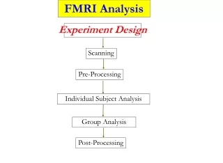
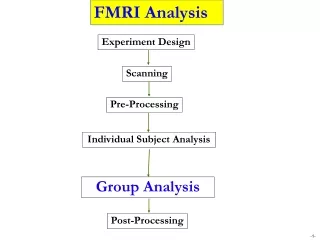
Group Analysis. File: afni24_GroupAna.pdf. Gang Chen SSCC/NIMH/NIH/HHS. Preview Introduction: basic concepts and terminology Why do we need to do group analysis? Factor, quantitative covariates, main effect, interaction, … G roup analysis approaches

E N D
Group Analysis File:afni24_GroupAna.pdf Gang Chen SSCC/NIMH/NIH/HHS
Preview • Introduction: basic concepts and terminology • Why do we need to do group analysis? • Factor, quantitative covariates, main effect, interaction, … • Group analysis approaches • t-test: 3dttest++ (3dttest), 3dMEMA • Regression: 3dttest++, 3dMEMA,3RegAna • ANOVA: 3dANOVAx, 3dMVM,GroupAna • ANCOVA or GLM: 3dttest++, 3dMEMA, 3dMVM, 3dLME • Impact & consequence of FSM, ASM, and ESM • Miscellaneous • Centering for covariates • Intra-Class Correlation (ICC) • Nonparametric approach, fixed-effects analysis • Inter-Subject Correlation (ISC)
Why Group Analysis? • Evolution of FMRI studies • Early days [1992-1994]: no need for group analysis • Seed-based correlation for one subject was revolutionary • Now: torture brain/data enough, and hope nature will confess! • Many ways to manipulate the brain (and data) • Reproducibility and generalization • Science strives for generality: summarizing subject results • Typically 10 or more subjects per group • Exceptions: pre-surgical planning, lie detection, … • Why not one analysis with a giant model for all subjects? • Computationally unmanageable and very hard to set up • Heterogeneity in data or experiment design across subjects • Model and data quality check at individual subject level
Simplest Group Analysis: One-Sample t-Test • SEM = Standard Error of the Mean = standard deviation of sample, divided by square root of number of samples = estimate of uncertainty in sample mean • One-sample t-test determines if sample mean is large enough relative toSEM Signal in Voxel, from 7 subjects (% change) +2 SEM 1 SEM 2 SEM one data sample = signal from one subject in this voxel in this condition Condition or Contrast of 2 conditions • statisticallysignificantly different from 0!
Simplest Group Analysis: Two-Sample t-Test • Group= some way to categorize subjects (e.g., sex, drug treatment, disease, …) • SEM = Standard Error of the Mean = standard deviation of sample divided by square root of number of samples = estimate of uncertainty in sample mean • Two-sample t-test determines if sample means are “far apart” compared to size of SEM Signal in Voxel, in each condition, from 7 subjects (% change) +2 SEM 1 SEM 2 SEM one data sample = signal from one subject in this voxel in this group Group # 1 Group # 2 • Not statistically significantly different!
paired data samples: same numbers as before Simplest Group Analysis: Paired (~1-sample) t-Test • Paired means that samples in different conditions should be linked together (e.g., from same subjects) • Test determines if differences between conditions in each pair are “large” compared to SEM of the differences • Paired test can detect systematic intra-subject differences that can be hidden in inter-subject variations • Lesson: properly separating inter-subject and intra-subject signal variations can be very important! • Essentially equivalent to one-sample t-test Signal paired differences Condition # 1 Condition # 2 • Significantly different! • Condition #2 #1, per subject
Toy example of group analysis • Responses from a group of subjects under one condition • : (β1, β2, …, β10)=(1.13, 0.87, …, 0.72) [% signal change] • Centroid: average (β1+β2+…+β10)/10 = 0.92 is not enough • Variation/reliability measure: diversity, spread, deviation • How different is 0.92 from 0 compared to its deviation? • Model building • Subject i‘s response = group average + deviation of subject i: simple model GLM (one-sample t-test) • If individual responses are consistent, should be small • How small (p-value)? • t-test: significance measure = • 2 measures: b (dimensional) and t(dimensionless)
Group Analysis Caveats • Results: two components (in afni GUI: OLay + Thr) • Effect estimates: have unit and physical meaning • Their significance (response to house significantly > face) • Very unfortunately p-values solely focused in FMRI! • Statistical significance (p-value) becomes obsession • Published papers: Big and tall parents (violent men, engineers) have more sons, beautiful parents (nurses) have more daughters • Statistical significance is not the same as practical importance • Fallacy: binarized thinking -- an effect that fails to reach statistical significance is not necessarily nonexistent • Statistically insignificant effect might be real • Sample size, suboptimal model, poor alignment across subjects
Group Analysis Caveats • Conventional: voxel-wise (brain) or node-wise (surface) • Prerequisite: reasonable alignment to some template • Limitations: alignment could be suboptimal or even poor • Different folding patterns across subjects: better alignment could help (perhaps to 5 mm accuracy?) • Different cytoarchitectonic (or functional) locations across subjects: structural alignment of images won’t help! • Impact on conjunction vs. selectivity • Alternative (won’t discuss): ROI-based approach • Half data for functional localizers, and half for ROI analysis • Easier: whole brain reduced to a few numbers per subject • Model building and tuning possible • Most AFNI 3d analysis programs also handle ROI input (1D files)
Group Analysis in NeuroImaging: why big models? Various group analysis approaches Student’s t-test: one-, two-sample, and paired ANOVA: one or more categorical explanatory variables (factors) GLM: AN(C)OVA LME: linear mixed-effects modeling Easy to understand: t-tests not always practical or feasible Tedious when layout (structure of data) is too complex Main effects and interactions: desirable Controlling for quantitative covariates Advantages of big models: AN(C)OVA, GLM, LME All tests in one analysis (vs. piecemeal t-tests): omnibus F Controlling for covariate effects Power gain: combining subjects across groups for estimates of signal and noise parameters (i.e., variances and correlations)
Terminology: Explanatory variables • Response/Outcome variable(HDR): regression βcoefficients • Factor: categorical, qualitative, descriptive, nominal, or discrete • Categorization of conditions/tasks • Within-subject (repeated-measures) factor • Subject-grouping: group of subjects • Between-subjects factor • Gender, patients/controls, genotypes, handedness, … • Subject: random factor measuring deviations • Of no interest, but served as random samples from a population • Quantitative(numeric or continuous) covariate • Three usages of ‘covariate’ • Quantitative value (rather than strict separation into groups) • Variable of no interest: qualitative (scanner, sex, handedness) or quantitative • Explanatory variable (regressor, independent variable, or predictor) • Examples: age, IQ, reaction time, brain volume, …
Terminology: Fixed effects • Fixed-effects factor: categorical (qualitative or discrete) variable • Treated as a fixed variable (constant to be estimated) in the model • Categorization of conditions/tasks (modality: visual/auditory) • Within-subject (repeated-measures) factor: 3 emotions • Subject-grouping: Group of subjects (gender, controls/patients) • Between-subject factor • All factor levelsare of interest: not interchangeable/replaceable • main effect, contrasts among levels • Fixed in the sense of statistical inferences • Apply only to the specific levels of the factor: : replacement test • Categories: human, tool • Don’t extend to other potential levels that might have been included (but were not) • Inferences from viewing human and tool categories can’t be generated to animals or clouds or Martians • Fixed-effects variable: quantitative covariate
Remember This Study? Tool motion (TM) Human whole-body motion (HM) Human point motion (HP) Tool point motion (TP) From Figure 1 Beauchamp et al. 2003 • 2 Factors, each with 2 levels • Factor A = type of object being viewed • Levels = Human or Tool • Factor B = type of display seen by subject • Levels = Whole or Points • This is repeated measures (4 βsper subject), 2 × 2 factorial
Terminology: Random effects • Random factor/effect • Random variable in the model: exclusively used for subject in FMRI • average + effects attributable to each subject: e.g. N(μ, τ2) • Requires enough subjects to estimate properly • Each individual subject effect is of NO interest: replacement test • Group response = 0.92%, subject 7 = 1.13%, random effect = 0.21% • Random in the sense • Subjects as random samples (representations) from a population • Inferences can be generalized to a hypothetical population • A generic group model: decomposing each subject’s response • Fixed (population) effects: universal constants (immutable): β • Random effects: individual subject’s deviation from the population (personality: durable for subject i): bi • Residuals: noise (evanescent): εi
Terminology: Omnibus tests - main effect and interaction • Main effect: any difference across levels of a factor? • Interactions: with ≥ 2 factors, interaction may exist • 2 × 2 design: F-test for interaction between A and B = t-test of (A1B1 - A1B2) - (A2B1 - A2B2) or (A1B1 - A2B1) - (A1B2 - A2B2) • t stastisticis better than F : a positive t shows A1B1 - A1B2 > A2B1 - A2B2 and A1B1 - A2B1 > A1B2 - A2B2
Terminology: Interaction • Interactions: ≥ 2 factors • May become very tedious to sort out or understand! • ≥ 3 levels in a factor • ≥ 3 factors • Solutions: reduction (in complexity) • Pairwise comparison • Plotting: ROI averages • Requires sophisticated modeling • AN(C)OVA: 3dANOVAx, 3dMVM, 3dLME • Interactions: quantitative covariates • In addition to linear effects, may have nonlinearity: y might depend on products of covariates: x1*x2, or x2
Terminology: Interaction • Interaction: between a factor and a quantitative covariate • Using explanatory variable (Age) in a model as a nuisance regressor(additive effect) may not be enough • Model building/tuning: Potential interactions with other explanatory variables? (as in graph on the right) • Of scientific interest (e.g., gender differences)
Models at Group Level • Conventional approach: taking β(or linear combination of multiple βs) only for group analysis • Assumption: all subjects have same precision (reliability, standard error, confidence interval) about β • All subjects are treated equally • Student t-test: paired, 1- and 2-sample: not random-effects models in strict sense (said to be random effects in Some other PrograM) • AN(C)OVA, GLM, LME • More precise method: taking both effect estimates and t-stats • t-statistic contains precision information about effect estimates • Each subject’s βis weighted based on precision of effect estimate (more precise βs get more weight) • Currently only available for t-test types
Piecemeal t-tests: 2 × 3 Mixed ANCOVA example A relatively simple model, but challenging for neuroimaging Factor A (Group): 2 levels (patient and control) Factor B (Condition): 3 levels (pos, neg, neu) Factor S (Subject): 15 ASD children and 15 healthy controls Quantitative covariate: Age Using Multiple t-tests for this study Group comparison + age effect Pairwise comparisons among three conditions Cannot control for age effect Effects that cannot be analyzed as t-tests Main effect of Condition (3 levels is beyond t-test method) Interaction between Group and Condition (6 levels total) Age effect across three conditions (just too complicated)
Classical ANOVA: 2 × 3 Mixed ANOVA Different denominator Factor A (Group): 2 levels (patient and control) Factor B (Condition): 3 levels (pos, neg, neu) Factor S (Subject): 15 ASD children and 15 healthy controls Covariate (Age): cannot be modeled; no correction for sphericity violation
Univariate GLM: 2 x 3 mixed ANOVA • Difficult to incorporate covariates • Broken orthogonality of matrix • No correction for sphericity violation a d b X Group: 2 levels (patient and control) Condition: 3 levels (pos, neg, neu) Subject: 3 ASD children and 3 healthy controls
Univariate GLM: popular in neuroimaging Advantages: more flexiblethan the method of sums of squares No limit on the the number of explanatory variables (in principle) Easy to handle unbalanced designs Covariates easily modeled when no within-subject factors present Disadvantages: costs paid for the flexibility Intricate dummy coding (to allow for different factors and levels) Tedious pairing for numerator and denominator of F-stat Choosing proper denominator SS is not obvious (errors in some software) Can’t generalize (in practice) to any number of explanatory variables Susceptible to invalid formulations and problematic post hoc tests Cannothandle covariates in the presence of within-subject factors No direct approach to correcting for sphericity violation Unrealistic assumption: same variance-covariance structure Problems: When overall residual SS is adopted for all tests F-stat: valid only for highestorder interaction of within-subject factors Most post hoc tests are inappropriate with this denominator
Univariate GLM: problematic implementations Correct Incorrect Between-subjects Factor A (Group): 2 levels (patient, control) Within-subject Factor B (Condition): 3 levels (pos, neg, neu) A) Omnibus tests B) Post hoc tests (contrasts) (1) Incorrectt-tests for factor A due to incorrect denominator (2) Incorrectt-tests for factor B or interaction effect AB when weights do not add up to 0 C) How to handle multiple βs per effect (e.g., multiple runs)? -- Artificially inflated DOF and assumption violation when multiple βs are fed into program
Univariate GLM: problematic implementations Correct Incorrect Within-subjects Factor A (Object): 2 levels (house, face) Within-subject Factor B (Condition): 3 levels (pos, neg, neu) A) Omnibus tests B) Post hoc tests (contrasts) (1) Incorrectt-tests for both factors A and B due to incorrect denominator (2) Incorrectt-tests for interaction effect AB if weights don’t add up to 0 C) How to handle multiple βs per effect (e.g., multiple runs)? -- Artificially inflated DOF and assumption violation when multiple βs are fed into program
Better Approach: Multivariate GLM Βn×m = Xn×qAq×m + Dn×m A D B B X Group: 2 levels (patient and control) Condition: 3 levels (pos, neg, neu) Subject: 3 ASD children and 3 healthy controls Age: quantitative covariate
Why use β , not t, values for group analysis? Why not use individual level statistics (t, F)? Dimensionless, no physical meaning Sensitive to sample size (number of trials) and to signal-to-noise ratio: may vary across subjects Are t-values of 4 and 100 (or p-values of 0.05 and 10-8) really informative? The HDR of the latter is not necessarily 25 times larger than the former Distributional considerations – not Gaussian β values Havephysical meaning: measure HDR magnitude = % signal change (i.e., how much BOLD effect) Using β values and their t-statistics at the group level More accurate approach: 3dMEMA Mostly about the same as the conventional (β only) approach Not always practical
Road Map: Choosing a program for Group Analysis? Starting with HDR estimated via shape-fixed method (SFM) One β per condition per subject It might be significantly underpowered (more later) Two perspectives Data structure Ultimate goal: list all the tests you want to perform Possible to avoid a big model this way Use a piecemeal approach with 3dttest++ or 3dMEMA Perform each test on your list separately Difficulty: there can be manytests you might want Most analyses can be done with 3dMVMand 3dLME Computationally inefficient Last resort: not recommended if simpler alternatives (e.g., t-tests) are available
Road Map: Student’s t-tests 3dttest++(new version of 3dttest) and 3dMEMA Not for F-tests except for ones with 1 DoFfor numerator All factors are of two levels (at most), e.g., 2 x 2, or 2 x 2 x 2 Scenarios One-, two-sample, paired Univariate GLM Multiple regression: 1 group + 1 or more quantitative variables ANCOVA: two groups + one or more quantitative variables ANOVA through dummy coding: all factors (between- or within-subject) are of two levels AN(C)OVA: multiple between-subjects factors + one or more quantitative variables: https://afni.nimh.nih.gov/sscc/gangc/MEMA.html One group against a constant: 3dttest/3dttest++ –singletonA The “constant” can depend on voxel, or be fixed
Road Map: between-subjects ANOVA One-way between-subjects ANOVA 3dANOVA 2 groups of subjects: 3dttest++, 3dMEMA (OK with > 2 groups too) Two-way between-subjects ANOVA Equal #subjects across groups: 3dANOVA2 –type 1 Unequal #subjects across groups: 3dMVM 2 x 2 design: 3dttest++, 3dMEMA(OK with > 2 groups too) Three-way between-subjects ANOVA 3dANOVA3–type 1 Unequal #subjects across groups: 3dMVM 2 x 2 design: 3dttest++, 3dMEMA(OK with > 2 groups too) N-way between-subjects ANOVA 3dMVM
Road Map: within-subject ANOVA Only one group of subjects One-way within-subject ANOVA 3dANOVA2–type 3 Two conditions: 3dttest++, 3dMEMA Two-way within-subject ANOVA 3dANOVA3–type 4 (2 or more factors, 2 or more levels each) 2 x 2 design: 3dttest++, 3dMEMA N-way within-subject ANOVA 3dMVM
Road Map: Mixed-type ANOVA and others One between- and one within-subject factor Equal #subjects across groups: 3dANOVA3–type 5 Unequal #subjects across groups: 3dMVM 2 x 2 design: 3dttest++, 3dMEMA More complicated scenarios Multi-way ANOVA: 3dMVM Multi-way ANCOVA (between-subjects covariates only): 3dMVM HDR estimated with multiple bases: 3dANOVA3, 3dLME, 3dMVM Missing data: 3dLME Within-subject covariates: 3dLME Subjects genetically related: 3dLME Trend analysis: 3dLME
One-Sample Case • One group of subjects (n ≥ 10) • One condition (visual or auditory) effect • Linear combination of multiple effects (visual vs. auditory) • Null hypothesis H0: average effect = 0 • Rejecting H0 is of interest! • Results • Average effect at group level (OLay) • Significance: t-statistic (Thr - Two-tailed by default in AFNI) • Approaches • uber_ttest.py (gen_group_command.py) – graphical interface • 3dttest++ • 3dMEMA
One-Sample Case: Example • 3dttest++: taking β only for group analysis 3dttest++ –prefix VisGroup-mask mask+tlrc-zskip \ -setA‘FP+tlrc[Vrel#0_Coef]’ \ ’FR+tlrc[Vrel#0_Coef]’ \ …… ’GM+tlrc[Vrel#0_Coef]’ • 3dMEMA: taking βand t-statistic for group analysis 3dMEMA –prefix VisGroupMEMA -mask mask+tlrc-setAVis \ FP ’FP+tlrc[Vrel#0_Coef]’’FP+tlrc[Vrel#0_Tstat]’ \ FR ’FR+tlrc[Vrel#0_Coef]’’FR+tlrc[Vrel#0_Tstat]’ \ …… GM ’GM+tlrc[Vrel#0_Coef]’ ’GM+tlrc[Vrel#0_Tstat]’ \ -missing_data 0 Voxel value = 0 treated it as missing Voxel value = 0 treated it as missing
Two-Sample Case • Two groups of subjects (n ≥ 10 each): males and females • One condition (e.g., visual or auditory) effect • Linear combination of multiple effects (e.g., visual minus auditory) • Example: Gender difference in emotional effect of stimulus? • Null hypothesis H0: Group1 = Group2 • Results • Group difference in average effect • Significance: t-statistic - Two-tailed by default in AFNI • Approaches • uber_ttest.py, 3dttest++, 3dMEMA • One-way between-subjects ANOVA • 3dANOVA: can also obtain individual group t-tests
Paired Case • One groups of subjects (n ≥ 10) • 2conditions (visual or auditory): no missing data allowed (3dLME) • Null hypothesis H0: Condition1 = Condition2 • Results • Average difference at group level • Significance: t-statistic (two-tailed by default) • Approaches • uber_ttest.py, gen_group_command.py,3dttest++, 3dMEMA • One-way within-subject (repeated-measures) ANOVA • 3dANOVA2 –type 3: can also get individual condition test • Missing data(3dLME): only 10 of 20 subjects have both βs • Essentially same as one-sample case using contrast as input
Paired Case: Example • 3dttest++: comparing two conditions 3dttest++ –prefix Vis_Aud \ -mask mask+tlrc–paired -zskip\ -setA’FP+tlrc[Vrel#0_Coef]’ \ ’FR+tlrc[Vrel#0_Coef]’ \ …… ’GM+tlrc[Vrel#0_Coef]’ \ -setB’FP+tlrc[Arel#0_Coef]’ \ ’FR+tlrc[Arel#0_Coef]’ \ …… ’GM+tlrc[Arel#0_Coef]’
Paired Case: Example • 3dMEMA: comparing two conditions using subject-level response magnitudes and estimates of error levels • Contrast should come from each subject • Instead of doing contrast inside 3dMEMA itself 3dMEMA –prefix Vis_Aud_MEMA \ -mask mask+tlrc-missing_data 0 \ -setA Vis-Aud \ FP ’FP+tlrc[Vrel-Arel#0_Coef]’’FP+tlrc[Vrel-Arel#0_Tstat]’ \ FR ’FR+tlrc[Vrel-Arel#0_Coef]’’FR+tlrc[Vrel-Arel#0_Tstat]‘ \ …… GM ’GM+tlrc[Vrel-Arel#0_Coef]’’GM+tlrc[Vrel-Arel#0_Tstat]’
One-Way Between-Subjects ANOVA • Two or more groups of subjects (n ≥ 10) • One condition or linear combination of multiple conditions • Example: visual, auditory, or visual vs. auditory • Null hypothesis H0: Group1 = Group2 • Results • Average group difference • Significance: t- and F-statistic (two-tailed by default) • Approaches • 3dANOVA (for more than 2 groups) • > 2 groups: pair-group contrasts: 3dttest++, 3dMEMA • Dummy coding: 3dttest++, 3dMEMA (hard work) • 3dMVM
Multiple-Way Between-Subjects ANOVA • Two or more subject-grouping factors: factorial designs • One condition or linear combination of multiple conditions • Examples: gender, control/patient, genotype, handedness • Testing main effects, interactions, single group, group comparisons • Significance: t- (two-tailed by default) and F-statistic • Approaches • Factorial design (imbalance not allowed): two-way (3dANOVA2 –type 1), three-way (3dANOVA3 –type 1) • 3dMVM: no limit on number of factors (imbalance OK) • All factors have two levels: 3dttest++, 3dMEMA • Using group coding (via covariates) with 3dttest++, 3dMEMA: imbalance possible
One-Way Within-Subject ANOVA • Also called one-way repeated-measures: one group of subjects (n ≥ 10) • Two or more conditions: extension to paired t-test • Example: happy, sad, neutral conditions • Main effect, simple effects, contrasts, general linear tests, • Significance: t- (two-tailed by default) and F-statistic • Approaches • 3dANOVA2 -type 3 (2-way ANOVA w/ 1 random factor) • With two conditions, equivalentto paired case with 3dttest++, 3dMEMA • With more than two conditions, can break into pairwise comparisons with 3dttest++, 3dMEMA • Univariate GLM: testing one condition is invalid
One-Way Within-Subject ANOVA • Example: visual vs. auditory condition 3dANOVA2 –type 3 -alevels 2 -blevels 10 \ -prefix Vis_Aud -mask mask+tlrc\ -amean 1 Vis –amean 2 Aud –adiff 1 2 V-A \ -dset 1 1 ‘FP+tlrc[Vrel#0_Coef]’ \ -dset 1 2 ‘FR+tlrc[Vrel#0_Coef]’ \ …… -dset 1 10 ’GM+tlrc[Vrel#0_Coef]’ \ -dset 2 1 ‘FP+tlrc[Arel#0_Coef]’ \ -dset 2 2 ‘FR+tlrc[Arel#0_Coef]’ \ …… -dset 2 10 ’GM+tlrc[Arel#0_Coef]’
Two-Way Within-Subject ANOVA • Factorial design; also known as two-way repeated-measures • 2within-subject factors • Example: emotion (happy/sad) and category (visual/auditory) • Testing main effects, interactions, simple effects, contrasts • Significance: t- (two-tailed by default) and F-statistic • Approaches • 3dANOVA3 –type 4 (three-way ANOVA with one random factor) • All factors have 2 levels (2x2): 3dttest++, 3dMEMA • Missing data? • Break into t-tests: 3dttest++, 3dMEMA • 3dLME
Two-Way Mixed ANOVA • Factorial design • One between-subjects and one within-subject factor • Example: between-subject factor = gender (male and female) and within-subject factor = emotion (happy, sad, neutral) • Testing main effects, interactions, simple effects, contrasts • Significance: t- (two-tailed by default) and F-statistic • Approaches • 3dANOVA3 –type 5 (three-way ANOVA with one random factor) • If all factors have 2 levels (2x2): 3dttest++, 3dMEMA • Missing data? • Unequal number of subjects across groups: 3dMVM, GroupAna • Break into t-tests: uber_ttest.py, 3dttest++, 3dMEMA • 3dLME
Univariate GLM: popular in neuroimaging Advantages: more flexiblethan the method of Sums of Squares (SS) No limit on the the number of explanatory variables (in principle) Easy to handle unbalanced designs Covariates can be modeled when no within-subject factors present Disadvantages: costs paid for the flexibility Intricate dummy coding – using covariates to partition βs into subsets Tedious pairing for numerator and denominator of F-stat Can be hard to select proper denominator SS Can’t generalize (in practice) to any number of explanatory variables Susceptible to invalid formulations and problematic post hoc tests Cannothandle covariates in the presence of within-subject factors No direct approach to correcting for sphericity violation Unrealistic assumption: same variance-covariance structure Problematic: When residual SS is adopted for all tests F-stat: valid only for highest order interaction of within-subject factors Most post hoc tests are inappropriate/invalid
MVM Implementation in AFNI Variable types Post hoc tests Program 3dMVM [written in R programming language] No tedious and error-prone dummy coding needed! Symbolic coding for variables and post hoc testing Data layout
Group analysis with multiple basis functions • Fixed-Shape method (FSM) • Estimead-Shape method (ESM) via basis functions: TENTzero, TENT, CSPLINzero, CSPLIN • Area under the curve (AUC) approach • Ignore shape differences between groups or conditions • Focus on the response magnitude measured by AUC • Potential issues: Shape information lost; Undershoot may cause trouble (canceling out some of the positive signal) • Better approach: maintaining shape information • Take individual β values to group analysis (MVM) • Adjusted-Shape method (ASM) via SPMG2/3 • Only take the major component βto group level • or, Reconstruct HRF, and take the effect estimates (e.g., AUC)
Group analysis with multiple basis functions • Analysis with effect estimates at consecutive time grids (from TENT or CSPLIN or reconstructed HRF) • Used to be considered very hard to set up (in GLM) • Extra variable in analysis: Time= t0, t1, …, tk • One group of subjects under one condition • Accurate null hypothesis is H0: β1=0, β2=0, …, βk=0 (NOTβ1=β2=…=βk) • Testing the centroid(multivariate testing) • 3dLME • Approximate hypothesis H0: β1=β2=…=βk (main effect) • 3dMVM • Result: F-statistic for H0 and t-statistic for each Time point
Group analysis with multiple basis functions • Multiple groups (or conditions) under one condition (or group) • Accurate hypothesis: • 2 conditions: 3dLME • Approximate hypothesis: • Interaction • Multiple groups: 3dANOVA3 –type 5 (two-way mixed ANOVA: equal #subjects), or 3dMVM • Multiple conditions: 3dANOVA3 –type 4 • Focus: do these groups/conditions have different response shape? • F-statistic for the interaction between Time and Group/Condition • F-statistic for main effect of Group: group/condition difference of AUC • F-statistic for main effect of Time: HDR effect across groups/conditions • Other scenarios: factor, quantitative variables • 3dMVM
Group analysis with multiple basis functions • 2 groups (children, adults), 2 conditions (congruent, incongruent), 1 quantitative covariate (age) • 2 methods: HRF modeled by 10 (tents) and 3 (SPMG3) bases
Group analysis with multiple basis functions • Advantages of ESM over FSM • More likely to detect HDR shape subtleties • Visual verification of HDR signature shape (vs. relying significance testing: p-values) • Study: Adults/Children with Congruent/Incongruent stimuli (2×2)