Visible-Surface Detection Methods
Visible-Surface Detection Methods Donald Hearn, M. Pauline Baker <Computer Graphics> 2001/08/03 Contents Abstract Introduction Back-Face Detection Depth-Buffer Method A-Buffer Method Scan-Line Method Depth-Sorting Method BSP-Tree Method Area-Subdivision Method Octree Method


Visible-Surface Detection Methods
E N D
Presentation Transcript
Visible-Surface Detection Methods Donald Hearn, M. Pauline Baker <Computer Graphics> 2001/08/03
Contents • Abstract • Introduction • Back-Face Detection • Depth-Buffer Method • A-Buffer Method • Scan-Line Method • Depth-Sorting Method • BSP-Tree Method • Area-Subdivision Method • Octree Method • Ray-Casting Method • Image-Space Method vs. Object-Space Method • Curved Surfaces • Wireframe Methods • Summary 2
Abstract • Hidden-surface elimination methods • Identifying visible parts of a scene from a viewpoint • Numerous algorithms • More memory - storage • More processing time – execution time • Only for special types of objects - constraints • Deciding a method for a particular application • Complexity of the scene • Type of objects • Available equipment • Static or animated scene 3 <Ex. Wireframe Displays>
Classification of Visible-Surface Detection Algorithms • Object-space methods vs. Image-space methods • Object definition directly vs. their projected images • Most visible-surface algorithms use image-space methods • Object-space can be used effectively in some cases • Ex) Line-display algorithms • Object-space methods • Compares objects and parts of objects to each other • Image-space methods • Point by point at each pixel position on the projection plane 5
Sorting and Coherence Methods • To improve performance • Sorting • Facilitate depth comparisons • Ordering the surfaces according to their distance from the viewplane • Coherence • Take advantage of regularity • Epipolar geometry • Topological coherence 6
Inside-outside test • A point (x, y, z) is “inside” a surface with plane parameters A, B, C, and D if • The polygon is a back face if • V is a vector in the viewing direction from the eye(camera) • N is the normal vector to a polygon surface N = (A, B, C) V 8
Advanced Configuration • In the case of concave polyhedron • Need more tests • Determine faces totally or partly obscured by other faces • In general, back-face removal can be expected to eliminate about half of the surfaces from further visibility tests <View of a concave polyhedron with one face partially hidden by other surfaces> 9
Characteristics • Commonly used image-space approach • Compares depths of each pixel on the projection plane • Referred to as the z-buffer method • Usually applied to scenes of polygonal surfaces • Depth values can be computed very quickly • Easy to implement Yv S3 S2 S1 (x, y) Xv 11 Zv
Depth Buffer & Refresh Buffer • Two buffer areas are required • Depth buffer • Store depth values for each (x, y) position • All positions are initialized to minimum depth • Usually 0 – most distant depth from the viewplane • Refresh buffer • Stores the intensity values for each position • All positions are initialized to the background intensity 12
Algorithm • Initialize the depth buffer and refresh buffer depth(x, y) = 0, refresh(x, y) = Ibackgnd • For each position on each polygon surface • Calculate the depth for each (x, y) position on the polygon • If z > depth(x, y), then set depth(x, y) = z, refresh(x, y) = Isurf(x, y) • Advanced • With resolution of 1024 by 1024 • Over a million positions in the depth buffer • Process one section of the scene at a time • Need a smaller depth buffer • The buffer is reused for the next section 13
Characteristics • An extension of the ideas in the depth-buffer method • The origin of this name • At the other end of the alphabet from “z-buffer” • Antialiased, area-averaged, accumulation-buffer • Surface-rendering system developed by ‘Lucasfilm’ • REYES(Renders Everything You Ever Saw) • A drawback of the depth-buffer method • Deals only with opaque surfaces • Can’t accumulate intensity values for more than one surface Foreground transparent surface Background opaque surface 15
Algorithm(1 / 2) • Each position in the buffer can reference a linked list of surfaces • Several intensities can be considered at each pixel position • Object edges can be antialiased • Each position in the A-buffer has two fields • Depth field • Stores a positive or negative real number • Intensity field • Stores surface-intensity information or a pointer value d > 0 I d < 0 Surf1 Surf2 Depth field Intensity field Depth field Intensity field (a) (b) <Organization of an A-buffer pixel position : (a) single-surface overlap (b) multiple-surface overlap> 16
Algorithm(2 / 2) • If the depth field is positive • The number at that position is the depth • The intensity field stores the RGB • If the depth field is negative • Multiple-surface contributions to the pixel • The intensity field stores a pointer to a linked list of surfaces • Data for each surface in the linked list • RGB intensity components • Opacity parameters(percent of transparency) • Depth • Percent of area coverage • Surface identifier • Pointers to next surface 17
Characteristics • Extension of the scan-line algorithm for filling polygon interiors • For all polygons intersecting each scan line • Processed from left to right • Depth calculations for each overlapping surface • The intensity of the nearest position is entered into the refresh buffer 19
Tables for The Various Surfaces • Edge table • Coordinate endpoints for each line • Slope of each line • Pointers into the polygon table • Identify the surfaces bounded by each line • Polygon table • Coefficients of the plane equation for each surface • Intensity information for the surfaces • Pointers into the edge table 20
Active List & Flag • Active list • Contain only edges across the current scan line • Sorted in order of increasing x • Flag for each surface • Indicate whether inside or outside of the surface • At the leftmost boundary of a surface • The surface flag is turned on • At the rightmost boundary of a surface • The surface flag is turned off 21
Example • Active list for scan line 1 • Edge table • AB, BC, EH, and FG • Between AB and BC, only the flag for surface S1 is on • No depth calculations are necessary • Intensity for surface S1 is entered into the refresh buffer • Similarly, between EH and FG, only the flag for S2 is on B E yv F Scan line 1 A S1 S2 Scan line 2 Scan line 3 H C D G xv 22
Example(cont.) • For scan line 2, 3 • AD, EH, BC, and FG • Between AD and EH, only the flag for S1 is on • Between EH and BC, the flags for both surfaces are on • Depth calculation is needed • Intensities for S1 are loaded into the refresh buffer until BC • Take advantage of coherence • Pass from one scan line to next • Scan line 3 has the same active list as scan line 2 • Unnecessary to make depth calculations between EH and BC 23
Drawback • Only if surfaces don’t cut through or otherwise cyclically overlap each other • If any kind of cyclic overlap is present • Divide the surfaces 24
Operations • Image-space and object-space operations • Sorting operations in both image and object-space • The scan conversion of polygon surfaces in image-space • Basic functions • Surfaces are sorted in order of decreasing depth • Surfaces are scan-converted in order, starting with the surface of greatest depth 26
Algorithm • Referred to as the painter’s algorithm • In creating an oil painting • First paints the background colors • The most distant objects are added • Then the nearer objects, and so forth • Finally, the foregrounds are painted over all objects • Each layer of paint covers up the previous layer • Process • Sort surfaces according to their distance from the viewplane • The intensities for the farthest surface are then entered into the refresh buffer • Taking each succeeding surface in decreasing depth order 27
Overlapping Tests • Tests for each surface that overlaps with S • The bounding rectangle in the xy plane for the two surfaces do not overlap (1) • Surface S is completely behind the overlapping surface relative to the viewing position (2) • The overlapping surface is completely in front of S relative to the viewing position (3) • The projections of the two surfaces onto the viewplane do not overlap (4) • If all the surfaces pass at least one of the tests, none of them is behind S • No reordering is then necessary and S is scan converted Easy Difficult 28
S S’ xv xv zv zv S S S’ S’ xv xv zv zv Overlapping Test Examples (1) (2) (3) (4) 29
S S’ S’’ S xv S’ zv xv zv Surface Reordering • If all four tests fail with S’ • Interchange surfaces S and S’ in the sorted list • Repeat the tests for each surface that is reordered in the list <S S’> <S S’’, then S’’ S’> 30
Drawback • If two or more surfaces alternately obscure each other • Infinite loop • Flag any surface that has been reordered to a farther depth • It can’t be moved again • If an attempt to switch the surface a second time • Divide it into two parts to eliminate the cyclic loop • The original surface is then replaced by the two new surfaces 31
Characteristics • Binary Space-Partitioning(BSP) Tree • Determining object visibility by painting surfaces onto the screen from back to front • Like the painter’s algorithm • Particularly useful • The view reference point changes • The objects in a scene are at fixed positions 33
Process • Identifying surfaces • “inside” and “outside” the partitioning plane • Intersected object • Divide the object into two separate objects(A, B) P1 P2 P1 C front back D A P2 P2 front back front back B front back A C B D back front 34
Characteristics • Takes advantage of area coherence • Locating view areas that represent part of a single surface • Successively dividing the total viewing area into smaller rectangles • Until each small area is the projection of part of a single visible surface or no surface • Require tests • Identify the area as part of a single surface • Tell us that the area is too complex to analyze easily • Similar to constructing a quadtree 36
Process • Staring with the total view • Apply the identifying tests • If the tests indicate that the view is sufficiently complex • Subdivide • Apply the tests to each of the smaller areas • Until belonging to a single surface • Until the size of a single pixel • Example • With a resolution 1024 1024 • 10 times before reduced to a point 37
Identifying Tests • Four possible relationships • Surrounding surface • Completely enclose the area • Overlapping surface • Partly inside and partly outside the area • Inside surface • Outside surface • No further subdivisions are needed if one of the following conditions is true • All surface are outside surfaces with respect to the area • Only one inside, overlapping, or surrounding surface is in the area • A surrounding surface obscures all other surfaces within the area boundaries from depth sorting, plane equation Surrounding Surface Overlapping Surface Inside Surface Outside Surface 38
Characteristics • Extension of area-subdivision method • Projecting octree nodes onto the viewplane • Front-to-back order Depth-first traversal • The nodes for the front suboctants of octant 0 are visited before the nodes for the four back suboctants • The pixel in the framebuffer is assigned that color if no values have previously been stored • Only the front colors are loaded 6 5 4 1 0 2 7 3 40
Displaying An Octree • Map the octree onto a quadtree of visible areas • Traversing octree nodes from front to back in a recursive procedure • The quadtree representation for the visible surfaces is loaded into the framebuffer 6 5 4 1 0 2 7 3 41 Octants in Space
Characteristics • Based on geometric optics methods • Trace the paths of light rays • Line of sight from a pixel position on the viewplane through a scene • Determine which objects intersect this line • Identify the visible surface whose intersection point is closest to the pixel • Infinite number of light rays • Consider only rays that pass through pixel positions • Trace the light-ray paths backward from the pixels • Effective visibility-detection method • For scenes with curved surfaces 43
Image-Space Method vs.Object-Space Method • Image-Space Method • Depth-Buffer Method • A-Buffer Method • Scan-Line Method • Area-Subdivision Method • Object-Space Method • Back-Face Detection • BSP-Tree Method • Area-Subdivision Method • Octree Methods • Ray-Casting Method 44
Abstract • Effective methods for curved surfaces • Ray-casting • Octree methods • Approximate a curved surface as a set of plane, polygon surfaces • Use one of the other hidden-surface methods • More efficient as well as more accurate than using ray casting and the curved-surface equation 46
Curved-Surface Representations • Implicit equation of the form • Parametric representation • Explicit surface equation • Useful for some cases • A height function over an xy ground plane • Scan-line and ray-casting algorithms • Involve numerical approximation techniques 47
Surface Contour Plots • Display a surface function with a set of contour lines that show the surface shape • Useful in math, physics, engineering, ... • With an explicit representation • Plot the visible-surface contour lines • To obtain an xy plot • Plotted for values of z • Using a specified interval z 48 <Color-coded surface contour plot>
Characteristics • In wireframe display • Visibility tests are applied to surface edges • Visible edge sections are displayed • Hidden edge sections can be eliminated or displayed differently from the visible edges • Procedures for determining visibility of edges • Wireframe-visibility(Visible-line detection, Hidden-line detection) methods 50