Download
1 / 29
290 likes | 460 Vues
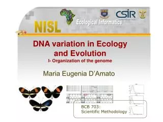
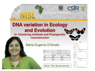
Maria Eugenia D’Amato. DNA variation in Ecology and Evolution II- Technical approach and concepts. BCB 703: Scientific Methodology. Methodological approaches to the study of genetic diversity. Molecular genetics techniques Types and properties of molecular makers

E N D
Maria Eugenia D’Amato DNA variation in Ecology and EvolutionII- Technical approach and concepts BCB 703: Scientific Methodology
Methodological approaches to the study of genetic diversity • Molecular genetics techniques • Types and properties of molecular makers • Factors that determine the patterns of genetic variation
Molecular techniques • Southern blot • PCR • DNA sequencing
Southern blot (1977) • Fragmentation of genomic • DNA in a reproducible way • 2. Separation of the fragments • in an electric field • 3. Transfer of the fragments from gel to • a membrane • 4. Probing of the membrane with known DNA • 5. Detection of the probe Sir Edwin Southern 1938- Nobel Price
Southern blot Restriction enzymes molecular scissors Southern blot steps
DNA fingerprinting Multilocus Trout DNA digested with Hinf I Unilocus (GATA)4 (GGAT)4 homozygote heterozygote
RFLPsRestriction Fragment Length Polymorphism. mtDNA PCR 500 250 500 bp Restriction site
PCR (1981) • Polymerase Chain Reaction • In vitro replication of DNA Kary Mullis 1938- Nobel Price 1993
PCR • DNA Copies = 2n, n = number of cycles • After 30 cycles: 107 million copies PCR machines
Applications of PCR:microsatellite genotyping priming site ♂ ♀ priming site x Pedigree analysis
Applications of PCRmicrosatellites for mating strategies Polyembryony in bryozoans? Incubating chamber
Applications of PCR. Anonymous loci AFLPs (Amplified Random Length Polymorphism) RAPDs (Random Amplified Polymorphic DNA) Dominant multilocus biallelic markers
DNA sequencing The old days…. Automatic sequencing A C G T CTCCGGCTGTAACCTTCAC…
Molecular Markers • Physical location in a genome whose inheritance can be monitored • polymorphic Parentage, relatedness, mating systems • Individual identification • Genic variation • Gene genealogies Gene flow, drift Phylogeography, speciation, deeper phylogenies
Genes in populations N N A p = 0.6 a p = 0.4 A a A a Aa AA pq A p = 0.6 p2 0.24 0.36 aa a p = 0.4 Aa pq q2 0.24 0.16
(p + q) 2 = p2 + 2pq + q2 Genes in populations:equilibrium of Hardy Weinberg p = freq A q = freq a the organism is diploid with sexual reproduction generations are non overlapping loci are biallelic allele frequencies are identical in males and females random mating population size is infinite no migration, no mutation, no selection Assumptions
Hardy Weinberg Equilibrium Consequences of the model • Allele frequencies remain constant, generation after generation • Genotype frequencies can be determined from allele frequencies
HWE- Mathematical example of deviation from equilibrium Expected genotype freqs In pop I: (0.6 + 0.4)2 = 0.62 + 2 x 0.6 x 0.4 + 0.42 = 0.36 + 0.48 + 0.16 2 = ∑ (O – E)2 2 = 44.4 d.f. = (R-1) x (C-1) = 2 2d.f =2 = 5.99 highly significant
1 2 3 4 5 6 7 8 9 Departures from HWE:Selection Charles Darwin Differential survival and reproductive success of genotypes Balancing selection Frequency dependent selection Directional selection 0.5 f ACER Normal and sickling forms of erythrocytes Heliconius erato sites
Deviations from HWE:Genetic drift • 2dqp0 q02N = • Random variation of allele frequencies • generation after generation • Generated by the random sampling process • of drawing gametes to form the next generation dq = q1 – q0 • Alleles become fixed (freq = 1) or lost (freq = 0) • The effect is more pronounced • in small populations • Genetic diversity decreases Variance in 1 generation
Genetic drift:Bottlenecks Original population Population crash recovery Cheetah: Late Pleistocene bottleneck American bison: Over hunting bottleneck
Genetic drift:Founder effect 1 couple carrying the allele immigrated SA in 1688 Today: 30 000 descendant South Africans are affected Skin photo-sensitivity in a porphyria patient
HWE departure/restorationMigration Migration = Gene flow transfer of alleles from one gene pool to another After m, 80% of the island is A1A1 and 20%A2A2 m Genotypes out of HWE A1A1 = 1 After 1 generation genotypes are in HWE A2A2 = 1
non random mating- drift – no gene flow Population structure • Differential allele frequencies between subpopulations • inbreeding coefficients : measure of H deficiency at • different hierarchical levels • Wahlund effect: H deficiency due to subdivision, drift • and inbreeding FIS = (Hs – Ho) / Ho within a subpopulation FIT = (HT – H0) / HT among individuals overall populations FST = (HS – HT) / HT between subpopulations Ho = aver. observed H within a subpopulation over loci Hs = aver. expected H within subpopulation over loci Ht = aver. expected H overall
Examples of population structure 1 Out of HWE 2 In HWE
Gene genealogies: a historical perspective Lineage: individuals or taxa related by a common ancestor Phylogenetic tree
Diversity with uniparental markers n haplotypes Haplotype diversity h = Total n individuals Nucleotide diversity n Σ xixjpij p = n -1
Phylogeography Population bottlenecks, expansions Gene flow Study of geographic distribution of lineages
ESUs Waples 1991: populations that are reproductively separate from other populations and have unique or different adaptations. Moritz 1994: populations that are reciprocally monophyletic for mtDNA alleles and show significant divergence of allele frequencies at nuclear loci. Crandall et al 2000 ecological exchangeability genetic exchangeability Reciprocal monophyly