Download
1 / 55
550 likes | 937 Vues
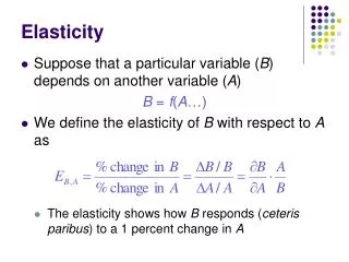
Elasticity Elasticity What do you think? Could reducing the supply of illegal drugs cause an increase in drug-related burglaries? Total Expenditure = P x Q S $2500 = $50 x 50 S’ $3200 = $80 x 40 S’ 80 S 50 D 40 50

E N D
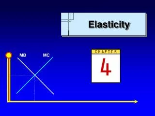
Elasticity • What do you think? • Could reducing the supply of illegal drugs cause an increase in drug-related burglaries? Chapter 4: Elasticity
Total Expenditure = P x Q S $2500 = $50 x 50 S’ $3200 = $80 x 40 S’ 80 S 50 D 40 50 e.g. 4.1 The Effect of Extra Border Patrols on the Market for Drugs How will drug addicts behave? P($/ounce) Q(1,000s of ounces/day) Chapter 4: Elasticity
Elasticity • Generally, elasticity is a measure of the responsiveness Chapter 4: Elasticity
Price Elasticity of Demand • is a measure of the responsiveness of the quantity demanded of a good to a change in the price of that good. • i.e. the percentage change in the quantity demanded that results from a 1 percent change in its price. Chapter 4: Elasticity
Example 4.2 • The price of beef increases by 2% and the quantity demanded decreases by 6% • Then the price elasticity of demand for beef is - 6% -3 = 2% Chapter 4: Elasticity
Price Elasticity of Demand • Measuring Price Elasticity of Demand • Observations • Price elasticity of demand will always be negative (i.e., an inverse relationship between price and quantity). • For convenience sometimes we drop the negative sign/ take absolute sign. Chapter 4: Elasticity
Price Elasticity of Demand Unit elastic inelastic Elastic Price elasticity of demand -3 -2 -1 0 Chapter 4: Elasticity
e.g 4.3elasticity of demand for dim sum? • Originally • Price = $10/piece • Quantity demanded = 600 pieces/day • New • Price = $9.5/piece • Quantity demanded = 606 pieces/day, then -1 (606 - 600)/600 1% = = (9.5 - 10)/10 -5% 5 Inelastic! Chapter 4: Elasticity
Example 4.4 What is the elasticity of Ocean Park Annual Passes? • Originally • Price = $1200 • Quantity demanded = 20,000 passes/year • New • Price = $1140 • Quantity demanded = 26,000 passes/year, then (26000 - 20000)/20000 30% = = -6 (1140 - 1200)/1200 -5% Elastic! Chapter 4: Elasticity
Determinants of Price Elasticity of Demand • Availability of substitutes More substitute to choose from when P of good X changes people can substitute X by other goods easily higher elasticity Chapter 4: Elasticity
Determinants of Price Elasticity of Demand • Proportion of income used to buy the good the higher the fraction of income spent on a good x higher elasticity as a slight increase in Px will affect your purchasing power adversely e.g. Housing Chapter 4: Elasticity
Determinants of Price Elasticity of Demand • Temporary versus permanent change in price if price change is temporary people react more to it higher elasticity e.g. Airline promotions Chapter 4: Elasticity
Determinants of Price Elasticity of Demand • Time facing a sudden price increases if we have more time to search for substitutes responsiveness higher higher elasticity e.g. marketing tactics Chapter 4: Elasticity
e.g 4.5 Price Elasticity Estimates for Selected Products Good or service Price elasticity Green peas -2.80 Restaurant meals -1.63 Automobiles -1.35 Electricity -1.20 Beer -1.19 Movies -0.87 Air travel (foreign) -0.77 Shoes -0.70 Coffee -0.25 Theater, opera -0.18 Why is the price elasticity of demand more than 14 times larger for green peas than for theater and opera performances? Chapter 4: Elasticity
A Graphical Interpretationof Price Elasticity • For small changes in price Where Q is the original quantity and P is the original price. Chapter 4: Elasticity
A P P P - P Q D Q Q + Q A Graphical Interpretationof Price Elasticity • For small changes in price Price Chapter 4: Elasticity
D A Example 4.6 Calculating Price Elasticity of Demand 20 16 12 Price 8 Question: What is the price elasticity of demand when P = $8? 4 1 2 3 4 5 Quantity Chapter 4: Elasticity
12 D1 6 4 D2 4 6 12 Example 4.7 Price Elasticity and Steepness of the Demand Curve What is the price elasticity of Demand for D1 & D2 when P = $4? P Observation If two demand curves have a point in common, the steeper curve must be less elastic with respect to price at that point. Q Chapter 4: Elasticity
a a/2 b/2 b Price Elasticity Regions along a Straight-Line Demand Curve Observation Price elasticity varies at every point along a straight-line demand curve Price Quantity Chapter 4: Elasticity
Example 4.8 Price Elasticity Regions along a Straight-Line Demand Curve When P = $4 When P = $1 12 6 Price Observation Price elasticity varies at every point along a straight-line demand curve 4 D 1 4 6 10 12 Quantity Chapter 4: Elasticity
Price Quantity Perfectly Elastic Demand Curve If the price increases a little, the quantity demanded will drop to zero. If the price drops a little, the quantity demanded will increase a lot. i.e. Consumers are extremely responsive to price changes Chapter 4: Elasticity
Price Quantity Perfectly Inelastic Demand Curve The quantity demanded is not responsive to any change in price. i.e. consumers are extremely inert to changes in price Chapter 4: Elasticity
Elasticity & Total Expenditure • From a consumer’s point of view, • Total Expenditure = P x Q • Market demand measures the quantity (Q) at each price (P) • Total Expenditure = Total Revenue (buyer’s view) (seller’s view) Chapter 4: Elasticity
12 10 8 6 Price ($/ticket) 4 2 0 1 2 3 4 5 6 Quantity (100s of tickets/day) Example 4.9 The Demand Curve for Drama Tickets Price ($/ticket) Total expenditure ($/day) 12 0 10 1000 8 1600 HIGHEST! 6 1800 4 1600 2 1000 0 0 Chapter 4: Elasticity
12 10 1,800 1,600 8 6 Price ($/ticket) 1,000 Total expenditure ($/day) 4 2 0 2 4 6 8 10 12 0 1 2 3 4 5 6 Price ($/ticket) Quantity (100s of tickets/day) Total Expenditure as a Function of Price Total revenue is at a maximum at the midpoint on a straight-line demand curve. Chapter 4: Elasticity
Example 4.10 • What happens to total expenditure on shelter when the price is reduced from $12/sq yd to $10/sq yd? • When P drop • Total Exp rise (fall) if gain from additional sales is larger (smaller) than loss from existing sales Chapter 4: Elasticity
Example 4.11 Elasticity and Total Expenditure • Should a jazz band raise or lower its price to increase total revenue? • Assume P=$20, Q=5,000, and e=-3. • Total revenue = $20 x 5,000 = $100,000/week • If P is increased 10%, • Q will decrease 30% • Total revenue = $22 x 3,500 = $77,000/week • If P is lowered 10%, • Q will increase 30% • Total revenue = $18 x 6,500 = $177,000/week Assume: Production Cost data is negligible in this case. Chapter 4: Elasticity
Elasticity and the Effect of a Price Change on Total Expenditure Chapter 4: Elasticity
Unitarily elastic demand curve P Unitary elastic: PxQ=constant all P, Q combinations yield the same TR for seller elasticity on all points= 1 Q Chapter 4: Elasticity
e.g. 4.12: should bus fare increases? • A director of a big bus company said, "For each 1 percent fare hike, we lose 0.2 percent of our riders." We can conclude that: a. a fare increase will increase total revenue. b. demand for bus service will go up as fares increase. c. demand is price elastic. d. a 10 percent fare hike will produce a 20 percent reduction in riders. e. the price elasticity is -5. Chapter 4: Elasticity
e.g. 4.12: should bus fare increases? • A director of a big bus company said, "For each 1 percent fare hike, we lose 0.2 percent of our riders." We can conclude that: • We are told that when DP/P = 1%, DQ/Q = -0.2%. • Elasticity = (DQ/Q)/(DP/P) = -0.2. (inelastic) So a fare increase will increase total revenue. Chapter 4: Elasticity
e.g. 4.12: should bus fare increases? • A director of a big bus company said, "For each 1 percent fare hike, we lose 0.2 percent of our riders." We can conclude that: a. a fare increase will increase total revenue. b. demand for bus service will go up as fares increase. c. demand is price elastic. d. a 10 percent fare hike will produce a 20 percent reduction in riders. e. the price elasticity is -5. answer a is correct. Chapter 4: Elasticity
Cross-Price Elasticity of Demand • The percentage by which quantity demanded of the good X changes in response to a 1 percent change in the price of the good Y • Substitute Goods • Complement Goods Chapter 4: Elasticity
Cross-Price Elasticity of Demand Substitute Goods • the cross-price elasticity of demand is positive • ‘positive’ = move in same direction • When Px ↑(↓) Qy ↑(↓) • E.g. Coffee & Tea Complement Goods • the cross-price elasticity of demand is negative • ‘negative’ = move in opposite direction • When Px ↓ (↑) Qy ↑(↓) • E.g. Coffee & Cream Chapter 4: Elasticity
Income Elasticity of Demand • The percentage by which quantity demanded changes in response to a 1 percent change in income • Normal Goods • Inferior Goods Chapter 4: Elasticity
Income Elasticity of Demand • Normal Goods • Income elasticity is positive • Income ↑(↓) Qx ↑(↓) • E.g. income and movie • Inferior Goods • Income elasticity is negative • Income ↓ (↑) Qx ↑(↓) • E.g. income and McDonalds (let’s assume you’re not a big fan…) Chapter 4: Elasticity
Now, the Supply Side So much for Demand side, let us change to the supply side discussion for elasticities Chapter 4: Elasticity
The Price Elasticity of Supply • Price Elasticity of Supply • The percentage change in the quantity supplied that occurs in response to a 1 percent change in price Chapter 4: Elasticity
S A 8 4 2 e.g. 4.13 A Supply Curve for Which Price Elasticity Declines as Quantity Rises B 10 8 • Observations: • Elasticity >0 • Elasticity >1 for linear supply curve that has a positive Y-intercept. • Elasticity decreases as quantity increases. Price 0 2 3 Quantity Chapter 4: Elasticity
S B 5 A 4 P Q Price 0 12 15 Quantity e.g. 4.14 A Supply Curve for Which Price Elasticity is unity The price elasticity of supply will always equal 1 at any point along a straight-line supply curve that passes through the origin. Chapter 4: Elasticity
S Elasticity = 0 at every point along a vertical supply curve Perfectly Inelastic Supply Curve What is the price elasticity of supply of land within Central? Price ($/acre) 0 Quantity of land in Central (1,000s of acres) Chapter 4: Elasticity
If Marginal Cost of production is constant, then the price elasticity of supply at every point along a horizontal supply curve is infinite More on Chapter 6 S A Perfectly Elastic Supply Curve Price (cents/cup) 14 0 Quantity of lemonade (cups/day) Chapter 4: Elasticity
Determinants of Supply Elasticity • Flexibility of inputs • Mobility of inputs • Ability to produce substitute inputs • Time Chapter 4: Elasticity
e.g.4:15 gasoline prices vs car prices • Why are gasoline prices so much more volatile than car prices? • Differences in markets • Demand for gasoline is more inelastic • Gasoline market has larger and more frequent supply shifts Chapter 4: Elasticity
S’ S 1.69 1.02 D 7.2 6 e.g.4:15 gasoline prices vs car prices Gasoline Greater Volatility in Gasoline Prices than in Car Prices Price ($/gallon) 0 Quantity (millions of gallons/day) Chapter 4: Elasticity
S’ S 17 16.4 D 11 12 e.g.4:15 gasoline prices vs car prices Greater Volatility in Gasoline Prices than in Car Prices Cars Price ($1,000s/car) Quantity (1,000s of cars/day) Cars Chapter 4: Elasticity
e.g.4:15 gasoline prices vs car prices • Conclusion: • Price will be more volatile when demand is more inelastic there are more frequent changes in the supply of that good Chapter 4: Elasticity
e.g.4.16 Beckham • Why does Beckham earn such an attractive income when compared to any soccer player? • Does he have a high or low price elasticity of supply of his services? His skills as a soccer player is a unique and essential inputs, an example of ultimate supply bottleneck. Chapter 4: Elasticity
Example 4.17 So why are the fares so different? If you start in Kansas City and you fly to Honolulu round-trip, the fare is a lot lower than if you start the same trip in Honolulu and fly to Kansas City round-trip. Passengers travel on same planes, consuming the same fuel, the same in-flight amenities, and so on. So why are the fares so different? By Karen Hittle, a student of Robert Frank. Chapter 4: Elasticity