Download
1 / 252
2.56k likes | 2.72k Vues
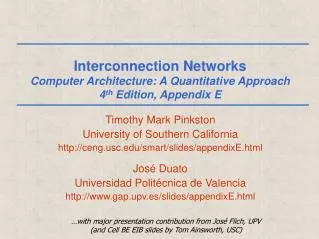
Interconnection Networks Computer Architecture: A Quantitative Approach 4 th Edition, Appendix E. Timothy Mark Pinkston University of Southern California http://ceng.usc.edu/smart/slides/appendixE.html José Duato Universidad Politécnica de Valencia

E N D
Interconnection NetworksComputer Architecture: A Quantitative Approach4th Edition, Appendix E Timothy Mark Pinkston University of Southern California http://ceng.usc.edu/smart/slides/appendixE.html José Duato Universidad Politécnica de Valencia http://www.gap.upv.es/slides/appendixE.html …with major presentation contribution from José Flich, UPV (and Cell BE EIB slides by Tom Ainsworth, USC)
Outline • E.1 Introduction (Lecture 1) • E.2 Interconnecting Two Devices (Lecture 1) • E.3 Interconnecting Many Devices (Lecture 2) • E.4 Network Topology (Lecture 2) • E.5 Network Routing, Arbitration, and Switching (Lecture 3) • E.6 Switch Microarchitecture (Lecture 4) • E.7 Practical Issues for Commercial Interconnection Networks (Lec 4) • E.8 Examples of Interconnection Networks (Lecture 5) • E.9 Internetworking (skipped) • E.10 Crosscutting Issues for Interconnection Networks (skipped) • E.11 Fallacies and Pitfalls (Lecture 5) • E.12 Concluding Remarks and References (Lecture 5)
End Node End Node End Node End Node Device Device Device Device … SW Interface SW Interface SW Interface SW Interface HW Interface HW Interface HW Interface HW Interface … … Link Link Link Link Introduction • How to connect individual devices together into a community of communicating devices? • Device (definition): • Component within a computer • Single computer • System of computers • Types of elements: • end nodes (device + interface) • links • interconnection network • Internetworking: interconnection of multiple networks Interconnection Network • Interconnection networks should be designed to transfer the maximum amount of information within the least amount of time (and cost, power constraints) so as not to bottleneck the system
Introduction • Reasons to devote attention to interconnection networks • They provide external connectivity from system to outside world • Also, connectivity within a single computer system at many levels • I/O units, boards, chips, modules and blocks inside chips • Trends: high demand on communication bandwidth • increased computing power and storage capacity • switched networks are replacing buses • Computer architects must understand interconnect problems and solutions in order to more effectively design and evaluate systems • Application domains • Networks implemented within processor chips and systems • Networks implemented across systems • Goal • To provide an overview of network problems and solutions • Examine a few case studies and examples
Introduction • Interconnection Network Domains • Interconnection networks can be grouped into four major networking domains, depending on the number and proximity of devices to be interconnected: OCNs, SANs, LANs, and WANs • On-chip networks (OCNs), a.k.a., network-on-chip (NoC) • Interconnect microarchitecture functional units, register files, caches, compute tiles, processor and IP cores • Chip or multichip modules • Tens (in future, possibly 100s) of devices interconnected • Maximum interconnect distance on the order of centimeters • Examples (custom designed) • Element Interconnect Bus (Cell Broadband Engine processor chip) • 2,400 Gbps (3.2 Ghz processor clock), 12 elements on the chip • Examples (proprietary designs) • CoreConnect (IBM), AMBA (ARM), Smart Interconnect (Sonic)
Introduction • Interconnection Network Domains • System/storage area networks (SANs) • Multiprocessor and multicomputer systems • Interprocessor and processor-memory interconnections • Server and data center environments • Storage and I/O components • Hundreds to thousands of devices interconnected • IBM Blue Gene/L supercomputer (64K nodes, each with 2 processors) • Maximum interconnect distance typically on the order of tens of meters, but some with as high as a few hundred meters • InfiniBand: 120 Gbps over a distance of 300 m • Examples (standards and proprietary) • InfiniBand, Myrinet, Quadrics, Advanced Switching Interconnect
Introduction • Interconnection Network Domains • Local area networks (LANs) • Interconnect autonomous computer systems • Machine room or throughout a building or campus • Hundreds of devices interconnected (1,000s with bridging) • Maximum interconnect distance on the order of few kilometers, but some with distance spans of a few tens of kilometers • Hundred devices (thousands with bridging) • Example (most popular): Ethernet, with 10 Gbps over 40Km • Wide area networks (WANs) • Interconnect systems distributed across the globe • Internetworking support is required • Many millions of devices interconnected • Maximum interconnect distance of many thousands of kilometers • Example: ATM
Introduction • Interconnection Network Domains WANs 5 x 10⁶ LANs 5 x 10³ Distance (meters) SANs 5 x 100 OCNs 5 x 10⁻³ 1 10 100 1,000 10,000 >100,000 Number of devices interconnected
Introduction • Organization • Top-down Approach • We unveil concepts and complexities involved in designing interconnection networks by first viewing the network as an ideal “black box” and then systematically removing various layers of the black box, exposing non-ideal behavior and complexities. • We first consider interconnecting only two devices (E.2) • We then consider interconnecting many devices (E.3) • Other layers of the black box are peeled away, exposing the network topology, routing, arbitration, and switching (E.4, E.5) • We then zoom in on the switch microarchitecture (E.6) • Next, we consider Practical Issues for Interconnection Networks (E.7) • Finally, we look at some examples: OCNs and SANs (E.8) • Internetworking (E.9) (skipped) • Additional Crosscutting Issues (E.10) (skipped) • Fallacies and Pitfalls (E.11) • Concluding Remarks (E.12) and References
Outline • E.1 Introduction (Lecture 1) • E.2 Interconnecting Two Devices (Lecture 1) • An Ideal Network • Network Interface Functions • Communication Protocol • Basic Network Structure and Functions • Characterizing Performance: Latency & Effective Bandwidth • Basic Network Characteristics in Commercial Machines • E.3 Interconnecting Many Devices (Lecture 2) • E.4 Network Topology (Lecture 2) • E.5 Network Routing, Arbitration, and Switching (Lecture 3) • E.6 Switch Microarchitecture (Lecture 4) • E.7 Practical Issues for Commercial Interconnection Networks (Lecture 4) • E.8 Examples of Interconnection Networks (Lecture 5) • E.9 Internetworking (skipped) • E.10 Crosscutting Issues for Interconnection Networks (skipped) • E.11 Fallacies and Pitfalls (Lecture 5) • E.12 Concluding Remarks and References (Lecture 5)
Interconnecting Two Devices • An Ideal Network • Two end node devices (A and B) • Device A (or B) may read an address in device B (or A) • Interconnection network behaves as dedicated links between A, B • Unidirectional wires each way dedicated to each device • Receiving buffers used for staging the transfers at the end nodes • Communication protocol: request, reply • basic functions at end nodes to commence and complete comm. int. network Device A Device B
to/from host Memory header trailer host interface Type checksum internal interconnect to/from network Network interface DMA FIFO DMA NIC Interconnecting Two Devices • Network Interface Functions • A message is the unit of information: header, payload, trailer • Interfacing to the network (hardware) • Communication device itself (OCNs and some SANs) • Additional network interface card or NIC (SANs, LANs, WANs) • Embedded processor(s), DMA engine(s), RAM memory Dest Information message payload NIC processor
header trailer Type checksum 00 = request 01 = reply 10 = request acknowledge 11 = reply acknowledge Interconnecting Two Devices • Network Interface Functions • Interfacing to the network (software, firmware) • Translate requests and replies into messages • Tight integration with operating system (OS) • Process isolation, protection mechanisms, etc. • Port (binds sender process with intended receiver process) • Packetization • Maximum transfer unit (MTU) used for dimensioning resources • Messages larger than MTU divided into packets with message id • Packet reordering at destination (for message reassembly) is done using sequence numbers Dest Info Msg ID Seq. # packet payload
Interconnecting Two Devices • Communication Protocol • Defines the sequence of steps followed by sender and receiver • Implemented by a combination of software and hardware • Hardware timers, CRC, packet processing, TLBs, ... • TCP off-load engines for LANs, WANs • OS-bypassing (zero-copy protocols) • Direct allocation of buffers at the network interface memory • Applications directly read/write from/to these buffers • Memory-to-memory copies avoided • Protection guaranteed by OS
Interconnecting Two Devices • Communication Protocol • Typical steps followed by the sender: • System call by application • Copies the data into OS and/or network interface memory • Packetizes the message (if needed) • Prepares headers and trailers of packets • Checksum is computed and added to header/trailer • Timer is started and the network interface sends the packets ni ni memory memory processor processor proc/mem bus IO bus or proc/mem bus IO bus or proc/mem bus proc/mem bus user space user space register file register file Interconnection network FIFO FIFO system space system space packet system call sends 1 copy pipelined transfer e.g., DMA user writes data in memory
Interconnecting Two Devices • Communication Protocol • Typical steps followed by the receiver: • NI allocates received packets into its memory or OS memory • Checksum is computed and compared for each packet • If checksum matches, NI sends back an ACK packet • Once all packets are correctly received • The message is reassembled and copied to user's address space • The corresponding application is signalled (via polling or interrupt) ni ni memory memory processor processor proc/mem bus IO bus or proc/mem bus IO bus or proc/mem bus proc/mem bus user space user space register file register file Interconnection network FIFO FIFO system space system space packet pipelined reception e.g., DMA interrupt 2 copy data ready
Interconnecting Two Devices • Communication Protocol • Additional stepsat the sender side: • ACK received: the copy is released and timer is cancelled • Timer expires before receiving an ACK: packet is resent and the timer is started ni ni memory memory processor processor user space user space register file register file Interconnection network pkt FIFO FIFO system space system space ACK
Interconnecting Two Devices • Communication Protocol • OS-bypassing (zero-copy or user-level protocols) • Direct allocation for DMA transfer to/from memory/NI buffers • Application directly reads/writes from/to these locations • Memory-to-memory copies are avoided • Protection is guaranteed by OS ni ni memory memory processor processor proc/mem bus IO bus or proc/mem bus IO bus or proc/mem bus proc/mem bus user space user space Interconnection network register file register file FIFO FIFO system space system space packet user copies data into pinned user space system call send. pipelined transfer e.g., DMA Pipelined peception e.g., DMA interrupt: data ready
processor processor proc/mem bus proc/mem bus register file register file Interconnecting Two Devices • Communication Protocol • OS-bypassing (zero-copy or user-level protocols) • Direct allocation for DMA transfer to/from memory/NI buffers • Application directly reads/writes from/to these locations • Memory-to-memory copies are avoided • Protection is guaranteed by OS • Is it possible to take out register to memory/buffer copy as well? ni ni memory memory IO bus or proc/mem bus IO bus or proc/mem bus user space user space Interconnection network FIFO FIFO system space system space packet
processor processor proc/mem bus proc/mem bus register file register file Interconnecting Two Devices • Communication Protocol • OS-bypassing (zero-copy or user-level protocols) • Direct allocation of system or network interface memory/buffers • Application directly reads/writes from/to these locations • Memory-to-memory copies are avoided • Protection is guaranteed by OS • Is it possible to take out register to memory/buffer copy as well? • NI buffer is associated with (or replaced by) register mapping ni ni Interconnection network FIFO FIFO packet Pipelined transfer
Interconnecting Two Devices • Raw’s 5-tuple Model (Taylor, et al. TPDS 2004): • Defines a figure of merit for operation-operand matching • End-to-end model: follows timing from sender to receiver • 5-tuple: <SO, SL, NHL, RL, RO> • SO: Send Occupancy • SL: Send Latency • NHL: Network Hop Latency • RL: Receive Latency • RO: Receive Occupancy • Conventional distr. SM MP: <10, 30, 5, 30, 40> • Raw / msg passing: < 3, 2, 1, 1, 7> • Raw / scalar: < 0, 1, 1, 1, 0> • ILDP: <0, n, 0, 1, 0>, (n = 0, 2) • Grid: <0, 0, n/8, 0, 0>, (n = 0..8) • Superscalar: < 0, 0, 0, 0, 0> “Scalar Operand Networks,” M. B. Taylor, W. Lee, S. P. Amarasinghe, and A. Agarwal, IEEE Trans. on Parallel and Distributed Systems , Vol. 16, No. 2, pp. 145–162, February, 2005.
Interconnecting Two Devices • Basic Network Structure and Functions • Media and Form Factor • largely depends on distance and signaling rate • up to centimeters (OCNs) • middle and upper copper metal layers at multi-gigabit rates • up to meters (SANs) • several layers of copper traces or tracks imprinted on circuit boards, midplanes, and backplanes at gigabit rates (differential-pair signaling); Cat 5 unshielded twisted-pair copper wiring • 100 meter distances (LANs) • Cat 5E unshielded twisted-pair copper wiring at 0.25 Gbps • Kilometer distances and beyond (WANs) • Coaxial copper cables at 10 Mbps • Optical media allows faster transmission speeds • Multimode and WDM techniques allow 100s to 1,000s Mbps
Interconnecting Two Devices • Basic Network Structure and Functions • Media and Form Factor OCNs SANs LANs WANs InfiniBand connectors Ethernet Metal layers Fiber Optics Media type Cat5E twisted pair Coaxial cables Printed circuit boards Myrinet connectors 10 100 0.01 1 >1,000 Distance (meters)
Interconnecting Two Devices • Basic Network Structure and Functions • Packet Transport • Hardware circuitry needed to drive network links • Encoding at the sender and decoding at the receiver • Multiple voltage levels, redundancy, data & control rotation (4b/5b) • Encoding—along with packet headers and trailers—adds some overhead, which reduces link efficiency • Physical layer abstraction: • viewed as a long linear pipeline without staging • signals propagate as waves through the transmission medium Tinjection < Tflight Tinjection = Tclk FIFO FIFO clk Tflight pipelined transfer
Interconnecting Two Devices • Basic Network Structure and Functions • Reliable deliveryof packets:lossy versus lossless networks • Must prevent the sender from sending packets at a faster rate than can be received and processed by the receiver • Lossy networks • Packets are dropped (discarded) at receiver when buffers fill up • Sender is notified to retransmit packets (via time-out or NACK) • Lossless networks (flow controlled) • Before buffers fill up, sender is notified to stop packet injection • Xon/Xoff (Stop & Go) flow control • Credit-based flow control (token or batched modes) • Implications of network type (lossless vs. lossy) • Constrains the solutions for packet routing, congestion, & deadlock • Affects network performance • The interconnection network domain dictates which is used • OCN, SAN: typically lossless; LAN, WAN: typically lossy
a packet is injected if control bit is in Xon Interconnecting Two Devices • Basic Network Structure and Functions • Xon/Xoff flow control Xon Xoff sender receiver Control bit Xoff Xon pipelined transfer
X Queue is not serviced Interconnecting Two Devices • Basic Network Structure and Functions • Xon/Xoff flow control When Xoff threshold is reached, an Xoff notification is sent When in Xoff, sender cannot inject packets Xon Xoff sender receiver Control bit Xoff Xon pipelined transfer
X Queue is not serviced Interconnecting Two Devices • Basic Network Structure and Functions • Xon/Xoff flow control When Xon threshold is reached, an Xon notification is sent Xon Xoff sender receiver Control bit Xoff Xon pipelined transfer
X Queue is not serviced Interconnecting Two Devices • Basic Network Structure and Functions • Credit-based flow control Sender sends packets whenever credit counter is not zero sender receiver Credit counter 10 9 8 6 5 1 3 2 4 0 7 pipelined transfer
X Queue is not serviced Interconnecting Two Devices • Basic Network Structure and Functions • Credit-based flow control Sender resumes injection Receiver sends credits after they become available sender receiver Credit counter 2 10 9 8 7 6 5 4 3 4 3 2 5 1 0 +5 pipelined transfer
Stop Stop Stop Stop Go Go Go Go Sender stops transmission Stop signal returned by receiver Last packet reaches receiver buffer Packets in buffer get processed Go signal returned to sender Sender resumes transmission First packet reaches buffer Stop & Go Time Sender uses last credit Last packet reaches receiver buffer Pacekts get processed and credits returned Sender transmits packets First packet reaches buffer # credits returned to sender Flow control latency observed by receiver buffer Credit based Time Interconnecting Two Devices • Basic Network Structure and Functions • Comparison of Xon/Xoff vs credit-based flow control Poor flow control can reducelink efficiency
Interconnecting Two Devices • Basic Network Structure and Functions • Example: comparison of flow control techniques • Calculate the minimum amount of credits and buffer space for interconnect distances of 1 cm, 1 m, 100 m, and 10 km • Assume a dedicated-link network with • 8 Gbps (raw) data bandwidth per link (each direction) • Credit-based flow control • Device A continuously sends 100-byte packets (header included) • Consider only the link propagation delay (no other delays or overheads) int. network Device A Device B Cr 8 Gbps raw data bandwidth
Packet size Packet propagation delay + Credit propagation delay ≤ х Credit count Bandwidth ( ) distance 100 bytes х 2 ≤ х Credit count 8 Gbits/sec 2/3 x 300,000 km/sec 1 cm → 1 credit 1 m → 1 credit 100 m → 10 credits 10 km → 1,000 credits Interconnecting Two Devices • Basic Network Structure and Functions • Example: comparison of flow control techniques int. network Device A Device B Cr 8 Gbps raw data bandwidth
Interconnecting Two Devices • Basic Network Structure and Functions • Error handling: must detect and recover from transport errors • Checksum added to packets • Timer and ACK per packet sent • Additional basic functionality needed by the protocol • Resolve duplicates among packets • Byte ordering (Little Endian or Big Endian) • Pipelining across operations
Interconnecting Two Devices • Characterizing Performance: Latency & Effective Bandwidth • Terms and Definitions: • Bandwidth: • Maximum rate at which information can be transferred (including packet header, payload and trailer) • Unit: bits per second (bps) or bytes per second (Bps) • Aggregate bandwidth: Total data bandwidth supplied by network • Effective bandwidth (throughput): fraction of aggregate bandwidth that gets delivered to the application • Time of flight: Time for first bit of a packet to arrive at the receiver • Includes the time for a packet to pass through the network, not including the transmission time (defined next) • Picoseconds (OCNs), nanoseconds (SANs), microseconds (LANs), milliseconds (WANs)
Interconnecting Two Devices • Characterizing Performance: Latency & Effective Bandwidth • Transmission time: • The time for a packet to pass through the network, not including the time of flight • Equal to the packet size divided by the data bandwidth of the link • Transport latency: • Sum of the time of flight and the transmission time • Measures the time that a packet spends in the network • Sending overhead (latency): • Time to prepare a packet for injection, including hardware/software • A constant term (packet size) plus a variable term (buffer copies) • Receiving overhead (latency): • Time to process an incoming packet at the end node • A constant term plus a variable term • Includes cost of interrupt, packet reorder and message reassembly
Sending overhead Transmission time (bytes/bandwidth) Time of flight Transmission time (bytes/bandwidth) Receiving overhead Transport latency Total latency packet size Latency = Sending Overhead + Time of flight + + Receiving Overhead Bandwidth Interconnecting Two Devices • Characterizing Performance: Latency & Effective Bandwidth Sender Receiver Time
int. network Device A Device B Cr 8 Gbps raw data bandwidth per link Interconnecting Two Devices • Characterizing Performance: Latency & Effective Bandwidth • Example (latency): calculate the total packet latencyfor interconnect distances of 0.5 cm, 5 m, 5,000 m, and 5,000 km • Assume a dedicated-link network with • 8 Gbps (raw) data bandwidth per link, credit-based flow control • Device A sends 100-byte packets (header included) • Overheads • Sending overhead: x + 0.05 ns/byte • Receiving overhead: 4/3(x) + 0.05 ns/byte • x is 0 μs for OCN, 0.3 μs for SAN, 3 μs for LAN, 30 μs for WAN • Assume time of flight consists only of link propagation delay (no other sources of delay)
Packet size LatencyOCN = 5 ns + 0.025 ns + 100 ns + 5 ns = 110.025 ns Latency = Sending overhead + Time of flight + + Receiving overhead Bandwidth LatencySAN = 0.305 μs + 0.025 ns + 0.1 μs + 0.405 μs = 0.835 μs LatencyLAN = 3.005 μs + 25 μs + 0.1 μs + 4.005 μs = 32.11 μs LatencyWAN = 20.05 μs + 25 μs + 0.1 μs + 40.05 μs = 25.07 ms int. network Device A Device B Cr 8 Gbps raw data bandwidth per link Interconnecting Two Devices • Characterizing Performance: Latency & Effective Bandwidth • Example (latency):
Sending overhead Receiving overhead Transport latency overlap time Interconnecting Two Devices • Characterizing Performance: Latency & Effective Bandwidth • Effective bandwidth with link pipelining • Pipeline the flight and transmission of packets over the links • Overlap the sending overhead with the transport latency and receiving overhead of prior packets “The Impact of Pipelined Channels on k-ary n-cube Networks ,” S. L. Scott and J. Goodman, IEEE Trans. on Parallel and Distributed Systems, Vol.5, No. 1, pp. 1–16, January, 1994.
Packet size BWLinkInjection = max (sending overhead, transmission time) Packet size BWLinkReception = max (receiving overhead, transmission time) 2 x Packet size Eff. bandwidth = min (2xBWLinkInjection , 2xBWLinkReception) = max (overhead, transmission time) overhead = max (sending overhead, receiving overhead) Interconnecting Two Devices • Characterizing Performance: Latency & Effective Bandwidth • Effective bandwidth with link pipelining • Pipeline the flight and transmission of packets over the links • Overlap the sending overhead with the transport latency and receiving overhead of prior packets (only two devices)
Determined by packet size, transmission time, overheads Ttransmission Tpropagation Treceiving Tsending Interconnecting Two Devices • Characterizing Performance: Latency & Effective Bandwidth • Characteristic performance plots: latency vs. average load rate; throughput (effective bandwidth) vs. average load rate Effective bandwidth Latency Peak throughput Peak throughput Average load rate Average load rate
Interconnecting Two Devices • Characterizing Performance: Latency & Effective Bandwidth • A Simple (General) Throughput Performance Model: • The network can be considered as a “pipe” of variable width • There are three points of interest end-to-end: • Injection into the pipe • Narrowest section within pipe (i.e., minimum network bisection that has traffic crossing it) • Reception from the pipe • The bandwidth at the narrowest point and utilization of that bandwidth determines the throughput!!! Reception bandwidth Bisection bandwidth Injection bandwidth
Effective bandwidth = min(BWNetworkInjection , BWNetwork , σ× BWNetworkReception) = min(N × BWLinkInjection , BWNetwork , σ× N × BWLinkReception) BWBisection BWNetwork = ρ× g Interconnecting Two Devices • σ is the ave. fraction of traffic to reception links that can be accepted (captures contention at reception links due to application behavior) • g is the ave. fraction of trafficthat must cross the network bisection • r is the network efficiency, which mostly depends on other factors: link efficiency, routing efficiency, arb. efficiency, switching eff., etc. • BWBisection is minimum network bisection that has traffic crossing it • Characterizing Performance: Latency & Effective Bandwidth • A Simple (General) Throughput Performance Model:
Effective bandwidth = min(BWNetworkInjection , BWNetwork , σ× BWNetworkReception) = min(2 × BWLinkInjection , BWNetwork , 1× (2 × BWLinkReception)) 2 ×BWLink BWNetwork = rL× 1 Interconnecting Two Devices • Characterizing Performance: Latency & Effective Bandwidth • Simple (General) Model Applied to Interconnecting Two Devices: rL= link efficiency resulting from flow control, encoding, packet header and trailer overheads Dedicated-link network int. network Device A BWLink Device B
int. network Device A Device B Cr BWLink = 8 Gbps raw data Interconnecting Two Devices • Characterizing Performance: Latency & Effective Bandwidth • Example: plot the effective bandwidth versus packet size • Assume a dedicated-link network with • 8 Gbps (raw) data bandwidth per link, credit-based flow control • Packets range in size from 4 bytes to 1500 bytes • Overheads • Sending overhead: x + 0.05 ns/byte • Receiving overhead: 4/3(x) + 0.05 ns/byte • x is 0 μs for OCN, 0.3 μs for SAN, 3 μs for LAN, 30 μs for WAN • What limits the effective bandwidth? • For what packet sizes is 90% of the aggregate bandwidth utilized? Dedicated-link network
> 655 bytes/packet for 90% utilization in SANs Interconnecting Two Devices • Characterizing Performance: Latency & Effective Bandwidth • Example: plot the effective bandwidth versus packet size All packet sizes allow for 90% utilization in OCNs Transmission time is the limiter for OCNs; overhead limits SANs for packets sizes < 800 bytes
Company System [Network] Name Intro year Max. compute nodes [x # CPUs] System footprint for max. configuration Packet [header] max. size Injection [Recept’n] node BW in Mbytes/s Minimum send/rec overhead Maximum copper link length; flow control; error Intel ASCI Red Paragon 2001 4,510 [x 2] 2,500 sq. feet 1984 B [4 B] 400 [400] few μsec handshaking; CRC+parity IBM ASCI White SP Power3 [Colony] 2001 512 [x 16] 10,000 sq. feet 1024 B [6 B] 500 [500] ~3 μsec 25 m; credit-based; CRC Intel Thunter Itanium2 Tiger4 [QsNetII] 2004 1,024 [x 4] 120 m2 2048 B [14 B] 928 [928] 0.240 μsec 13 m;credit- based; CRC for link, dest Cray XT3 [SeaStar] 2004 30,508 [x 1] 263.8 m2 80 B [16 B] 3,200 [3,200] few μsec 7 m; credit- based; CRC Cray X1E 2004 1,024 [x 1] 27 m2 32 B [16 B] 1,600 [1,600] ~0 (direct LD/ST acc.) 5 m; credit- based; CRC IBM ASC Purple pSeries 575 [Federation] 2005 >1,280 [x 8] 6,720 sq. feet 2048 B [7 B] 2,000 [2,000] ~ 1 μsec * 25 m; credit- based; CRC IBM Blue Gene/L eServer Sol. [Torus Net] 2005 65,536 [x 2] 2,500 sq. feet (.9x.9x1.9 m3/1K node rack) 256 B [8 B] 612,5 [1,050] ~ 3 μsec (2,300 cycles) 8.6 m; credit- based; CRC (header/pkt) Interconnecting Two Devices • Basic Network Characteristics of Commercial Machines *with up to 4 packets processed in parallel
Outline • E.1 Introduction (Lecture 1) • E.2 Interconnecting Two Devices (Lecture 1) • E.3 Interconnecting Many Devices (Lecture 2) • Additional Network Structure and Functions • Shared-Media Networks • Switched-Media Networks • Comparison of Shared- versus Switched-Media Networks • Characterizing Performance: Latency & Effective Bandwidth • E.4 Network Topology (Lecture 2) • E.5 Network Routing, Arbitration, and Switching (Lecture 3) • E.6 Switch Microarchitecture (Lecture 4) • E.7 Practical Issues for Commercial Interconnection Networks (Lec 4) • E.8 Examples of Interconnection Networks (Lecture 5) • E.9 Internetworking (skipped) • E.10 Crosscutting Issues for Interconnection Networks (skipped) • E.11 Fallacies and Pitfalls (Lecture 5) • E.12 Concluding Remarks and References (Lecture 5)
Interconnecting Many Devices • Additional Network Structure and Functions • Basic network structure and functions • Composing and processing messages, packets • Media and form factor • Packet transport • Reliable delivery (e.g., flow control) and error handling • Additional structure • Topology • What paths are possible for packets? • Networks usually share paths among different pairs of devices • Additional functions (routing, arbitration, switching) • Required in every network connecting more than two devices • Required to establish a valid path from source to destination • Complexity and applied order depends on the category of the topology: shared-media or switched media