Methods for Simulating Discrete Stochastic Chemical Reactions
360 likes | 497 Vues
Methods for Simulating Discrete Stochastic Chemical Reactions. Tuesday, Nov 9, 2010. Exact stochastic algorithm Tau-leap algorithm Chemical langevan equation. Discrete Stochastic Simulations (Chemical Reactions).

Methods for Simulating Discrete Stochastic Chemical Reactions
E N D
Presentation Transcript
Methods for Simulating Discrete Stochastic Chemical Reactions Tuesday, Nov 9, 2010 Exact stochastic algorithm Tau-leap algorithm Chemical langevan equation
Discrete Stochastic Simulations(Chemical Reactions) • We consider here the situation where different chemical can react with each other, governed by different reactions. In fact, the “chemicals” can be molecules, cells, or even organisms, and the “reactions” can be any interaction rules. • We consider the situation where there are such a small number of chemicals that the stochastic element becomes significant. • However, these methods are restricted to systems of uniformly mixed chemicals.
Chemical Reactions as a Poisson Process • Under these assumptions, chemical reactions are a Poisson process, meaning each reaction occurs stochastically at a rate dependent only on the current state of the system, not dependent on previous states or events. • This is also called a memoryless process • We will look at several methods to simulate this. • In what conditions does each provide accurate results? • How efficient is each?
Four Views of a Poisson Process: • If the rate of an event is l, then, t = 1/l is mean time to next event. • We consider four ways to step through time for a Poisson process • What is probability that an event will occur in time T << t ? This is inefficient and we don’t use it. • At what time does the next event occur? • How many events occur in time T ~> t? • How many events occur in time T >> t?
Three Ways to Simulate a Poisson Process: • Match time step to next event (1 event) • Gillespie’s “exact” algorithm • Always accurate, but moderately expensive • Take medium time steps (0 to ~20 events) • “Tau-leap” algorithm • less expensive and reasonably accurate if system doesn’t change in a time step (so if time step is well chosen); • Take large time steps (> 10 events) • Gillespie’s “Chemical Langevin Equation” algorithm • Accurate if system doesn’t change in a time step, but > 10 events occur. Least expensive
Reaction-Based Solving Methods: • Is converted to • dX/dt = -aXY; • dY/dt = -aXY +bZ; • dZ/dt = aXY-bZ; • We are used to writing differential equations from chemical reactions. • For example: • X+Y Z (rate a) • Z Y (rate b) • But in stochastic systems the actual “events” or “reactions” is stochastic. • And, when a reaction occurs, it affects many “chemicals” at once. • So uncertainty in these chemicals is coupled. • Thus, need to organize algorithms on the number and type of reactions that occur, not on the change in each chemical, as we are used to.
Uniform Formalism: • Reaction-Based Solving Methods: • Gillespie exact algorithm • Tau-leap • Chemical Langevin equation • There are three publications that present these methods. • Different methods and uses, but also different formalisms, yet the underlying methods are very similar. • Wendy’s unified formalism: • We present each of them with the same formalism, to make both understanding and implementation easier, but this will not exactly match the original papers.
Unified Formalism: • Reactions • R reactions with r as the index. • (always presented as different rows in matrices) • Chemicals • C chemicals with c as the index • (always presented as different columns in matrices) • Chemicals on left of equation are called substrates • Chemicals on right of equation are called products E+S ES E + S E + P ES E + P • k are the rate constants for each reaction • k(r) or kr is the rate constant for the rth reaction.
Define System: • Define R reactions according to stoichiometry using two matrices and a column vector: • Matrix S is the substrates. • Matrix P is the products. • Vector K is the reaction rates. • Example: S1 + S2 S3 with rate constant k1 S1 + S1 S2 with rate constant k2, S = [1, 1, 0; P = [0, 0, 1; K = [k1 2, 0, 0]; 0, 1, 0]; k2]; • Initial conditions: X(0) for C chemicals: [X1, X2, …XC]
Gillespie AlgorithmStochastic Simulation Alogorithm • Exact Algorithm to solve chemical reactions • Essentially mimics real situation: • Given rates and molecule numbers, • How long until next change occurs? • Which is next event that occurs? • Elegant and simple. Proposed in 1977 • Still used today.
Step 1:Given the system state, determine the rate of each reaction, ar. • Reaction 1: S1 + S2 S3, with rate constant k1 • X1, X2 are the numbers of the reactant molecules • Define the stoichiometry: h1 = X1X2 ; this will give dependence on amounts of molecules. • Then a1= h1k1= k1 X1X2 = rate for this reaction. • Reaction 2: S1 + S1 S2, • h2 = X1(X1-1)/2 (why is this true?) • Finally, define: a0 = ar (r = 1 to R) • This is the combined rate of all possible reactions
Gillespie Rates: What is the residence time of this state? How fast do we leave this state? a1 aR x1, x2, ..xC aR-1 a2 a0 = ar (r = 1 to R) is the total rate at which some reaction occurs. ar
What is the residence time of this state? Probability p that state still survives at time t: Simple Poisson Process Current state x1, x2, ..xR Exponential decay Thus: a0 All other states As p decays from 1 to 0, t increases from 0 to infinity
Step 2 When does the next reaction occur … Pick p, a uniform random number from 0 to 1 Let This is time of the next event. (Note that the time step doesn’t have to be predetermined, and is exact.)
a1 a2 a3 a4 Step 2 …and which reaction is it? • Determine which reaction occurs at time t: • Pick p2, another uniform random number from 0 to 1 • Find r, such that: • Think about dividing a0 into R pieces of length ar • p2 determines r based on weighting: p2a0
Step 3 Update the System State • Update t = t + t • Update X = [X1, X2, …XC] according to the reaction stoichiometry • Subtract substrates and add products for the indicated rth reaction. • For each c, Xc = Xc – S(r,c) + P(r,c) • In matrix format: • X(end+1,:) = X(end,:) – S(r,:) + P(r,:) • Update reaction step counter (RC = RC+1). Step 3 is to determine how each of C chemicals are affected
Questions? • Why is (on average) the time to the next step the same, whether the actual event has a slow or fast rate? • Example: student state change in class.
Collecting Data From Gillespie • The algorithm writes out [X1, X2, …XC, t] at each time step. • But all the runs will encounter different time steps, and likely more than you need! • Make a time vector: • time = linspace(0,totalTime,100); • After each run, calculate data at periodic intervals with interp1: • Y(1,:)= interp1(t,X(1,:),time,'nearest'); • Calculate mean values and variance just like previous examples
Advantages of Gillespie • Exact simulation; doesn’t make linear approximation of probability = a0Dt. • This means that time steps can be longer; Dt (simple time step) << t (Gillespie time step) • No need to predetermine time steps • Time step responds to changes in rates as numbers of particles change. • No conditions: always is accurate.
Disadvantages of Gillespie • Gets very slow when any one reaction is very fast relative to others. (stiff systems) • Fast reaction occurs with fast rates or if there are a lot of a reactant. • Thus, can be ineffective even though it is accurate in theory. • Tau-leap algorithm deals with these situations
Four Ways to Simulate a Poisson Process: • Take tiny time steps (last Tuesday) (<<1 events) • “simple” algorithm • Always accurate if time step is small enough but very expensive. Safe time step may depend on state. • Match time step to next event (1 event) • Gillespie’s “exact” algorithm • Always accurate, but moderately expensive • Take medium time steps (0 to ~20 events) • “Tau-leap” algorithm • Accurate if system doesn’t change in a time step; less expensive • Take large time steps (> 10 events) • Gillespie’s “Chemical Langevin Equation” algorithm • Accurate if system doesn’t change in a time step, but > 10 events occur. Least expensive
Tau-leap method • Explained in Higham 2007 article, page 12 • When using the exact stochastic algorithm, time for next reaction is determined. • When there are lots of some type of chemical, you don’t need to take so few steps for reactions involving this chemical, since your system doesn’t change much anyway. • Tau-leap: • for a given size of time step, • determine the number of each reaction that occur in that time step using the Poisson distribution • update all reactions simultaneously • Assumes: system (rates) doesn’t change much in one time step (like all ODEs).
Expected Number of Events: • Like Gillespie: • The rate that each reaction r occurs is ar • It is calculated the exact same way. • Unlike Gillespie: • For each r, ask: how many reactions will take place in time Dt? • Expected value is lr = arDt. • Recall: Poisson distribution: what is the probability of getting n when the expected value is l? • (Why don’t we use the binomial distribution to make sure we don’t use up a reagent?)
Algorithm for actual number of events: • From last slide, have calculated the expected value l • Pick r, a random number between 0 and 1, uniform distribution. • Psum = 0 • In a loop starting at n = 0 Calculate P(n) given lr from Psum = Psum + P(n) if r < Psum, then nr = n; exit loop • n gives how many of this reaction occurs. • Do this for each reaction! • I have written a function, n = randp(lambda), that does just this. It is called by the TauLeapWendy algorithm.
Update the System State: • On last two slides, for each reaction: • Calculated estimated number of reactions, lr • Calculated the actual number of reactions, nr • Then, update values of each chemical c by using the reaction stoichiometry multiplied by nr • In matrix format: X(end+1,:) = X(end,:)+ n*(-S + P); Where n is a vector of the nr.
How to Determine the Time Step? • Choice 1: fix the time step throughout the simulation (easy, but inaccurate and/or inefficient) • Choice 2: adjustable time step depends on system state (accurate and efficient) • To do this, want largest time step that isn’t expected to change the system state. • Must decide this BEFORE finding the random numbers • Otherwise, will bias towards smaller changes • Thus must use the EXPECTED fractional change • Change = lambda*(-S + P); • Current = X(end,:) • Consider: Max(abs(change./current)) • If > RelTol, make step smaller. • Some mechanism to increase step
Tau-leap • Step 0: set up S,P,K • Step 1: Calculate • ar • lr = arDt • (adjust time step until OK) • Step 2: use R random numbers to determine number of events, nr , for each reaction. • Step 3: update system for all R reactions Gillespie • Step 0: set up S,P,K • Step 1: Calculate ar a0 =sum(ar) • Step 2: Use 2 random numbers to pick when the next occurs and which reaction it is. • Step 3: update system for the one reaction only
Conditions for tau-leap • Condition: Require Dt to be small enough that so the system doesn’t change appreciably during that step (same as any deterministic ODE solver)
Four Ways to Simulate a Poisson Process: • Take tiny time steps (last Tuesday) (<<1 events) • “simple” algorithm • Always accurate if time step is small enough but very expensive. Safe time step may depend on state. • Match time step to next event (1 event) • Gillespie’s “exact” algorithm • Always accurate, but moderately expensive • Take medium time steps (0 to ~20 events) • “Tau-leap” algorithm • Accurate if system doesn’t change in a time step; less expensive • Take large time steps (> 10 events) • Gillespie’s “Chemical Langevin Equation” algorithm • Accurate if system doesn’t change in a time step, but > 10 events occur. Least expensive
Chemical Langevin Equations • A way to simulate chemical reactions where numbers of elements are • large enough to use continuous model, • but small enough to consider stochastic process • Name and method are motivated by the Langevin Equation for diffusion.
Poisson Random Process a1 is reaction rate • Recall that a Poisson distribution is: • How many events occur in time Dt? • Expected value is: • Variance = mean, so • The CENTRAL LIMIT THEOREM states • The sum of a sufficiently large number of independent random variables of identical distribution (like the bournoulli distribution) has an approximately normal distribution • Thus, if a1Dt > ~10, can use: • P(k) = N(a1Dt, a1Dt) • Read: normal distributed with mean a1Dt and variance a1Dt.
Daniel Gillespie 2000,Chemical Langevin Equation (CLE) Wendy Formalism: Exactly like tau-leap, but use alternate way to get n from lambda = a1Dt Gillespie: J. Chem Phys, Vol. 113, pp. 297–306, (2000)
Normally Distributed Random Variables in MATLAB r=randn; Gives normally distributed random variable with mean 0 and standard deviation 1. r=mu+simga*randn; Gives normally distributed random variable with mean mu and standard deviation sigma.
Concentrations vs Numbers Note that am(xt)Dt is how much the system would change in a deterministic equation due to the reaction m. We work in numbers and not concentrations because the noise depends on number, not standard deviations. But second-order rate constants still require a concentration so volume also must be known. If volume is constant, this can be incorporated into cm.
Conditions for Chemical Langevin • Condition 1: Require Dt to be small enough that so the system is not expected to change appreciably during that step (same as tau-leap, and any deterministic ODE solver) • Condition 2: Require Dt to be large enough that the expected number of occurrences of each reaction is much larger than 1, so continuous approximation is acceptable. (Unique to CLE) • Wendy approach: Pick time step to meet condition 1, and use CLE for each reaction if condition 2 is met, tau-leap if not.
Gillespie exact, tau-leap, Chemical LangevanAlgorithmic Notes • All three methods are reaction-based. • Use S, P, and K for stoichiometry and rate constants • Exact is more accurate • A combination of Tau-leap and CLE, (in which normal distribution replaces Poisson when expected number > 15) is faster for certain systems (but can be slower for others).