Chaos in a Pendulum Section 4.6
230 likes | 548 Vues
Chaos in a Pendulum Section 4.6. To introduce chaos concepts , use the damped , driven pendulum. This is a prototype of a nonlinear oscillator which can display chaos. The Pendulum The nonlinearity has been known for hundreds of years.

Chaos in a Pendulum Section 4.6
E N D
Presentation Transcript
Chaos in a PendulumSection 4.6 • To introduce chaos concepts, use the damped, driven pendulum. This is a prototype of a nonlinear oscillator which can display chaos. The Pendulum • The nonlinearity has been known for hundreds of years. • Thoroughly discussed (for the undamped case!) in Sect. 4.4. • Chaotic behavior in pendula has only been discovered (& explored) recently (20-30 years).
Some pendulum systems for which the motion has been found to be chaotic: Support undergoing forced sinusoidal oscillations Double pendulum
Coupled pendula Magnetic pendulum
(sinusoidal) • We aren’t going to analyze these! • Instead, as a prototype for pendula which exhibit chaos, go back to the ordinary plane pendulum we’ve already seen, but add a sinusoidal driving force and a damping term
Equation of motion(rotational version of Newton’s 2nd Law): Total torque about the axis = (moment of inertia) (angular acceleration) Assume a damping torque proportional to the angular velocity & sinusoidal driving torque: N = I(d2θ/dt2) = - b(dθ/dt) - mgsinθ + Nd cos(ωdt) Divide by I = m2 & define B (b/I), (ω0)2 (g/), D (Nd/I) ω0 Natural frequency for small θ of (“simple”) pendulum (d2θ/dt2) = -B(dθ/dt) – (ω0)2 sinθ + D cos(ωdt)
For ease of numerical solution, go to dimensionless variables. • Divide the equation of motion by the natural frequency squared: (ω0)2 (g/), Define the dimensionless variables: Time:t ω0t (g/)½t Oscillating variable: x θ Driving frequency: ω(ωd/ω0) (/g)½ωd Damping constant:c b/(m2ω0) b/(mg) Driving force (torque) strength: F Nd/(m2ω0) Nd/(mg)
Also note that: x = (dx/dt) = (dθ/dt)(dt/dt) = (dθ/dt)(ω0)-1 = θ(ω0)-1 x = (d2x/dt2) = (d/dt)[(dθ/dt)(ω0)-1] = (d2θ/dt2)(ω0)-2 = θ(ω0)-2 • So, the equation of motion finally becomes: x + cx + sin(x) = F cos(ωt) • A nonlinear driven oscillator equation! The author used numerical methods to solve for x(t) for various values of the parameters c, F, ω
To solve this numerically, its first convert this 2nd order differential equation to two 1st order differential equations! x + cx + sin(x) = F cos(ωt).DEFINE: y (dx/dt) = x (angular velocity),z ωt (dy/dt) = - cy – sin(x) + F cos(z) • Results are shown in the rather complicated figure (next page), which we’ll now look at in detail! For c = 0.05, ω = 0.7, results are shown for (driving torque strength) F = 0.4, 0.5, 0.6, 0.7, 0.8, 0.9 • Bottom line of the results from the figure: 1. The motion is periodic for F = 0.4, 0.5, 0.8, 0.9 2. The motion is chaoticfor F = 0.6, 0.7, 1.0 • This indicates the richness of the results which can come from nonlinear dynamics! This is surprising only if you think linearly! Thinking linearly, one would expect the solution for F = 0.6 to not be much different from that for F = 0.5, etc.
F = 0.8 • Left figure shows y (dx/dt)(angular velocity)vs time tat steady state (transient effects have died out). F = 0.4 ~ simple harmonic motion F = 0.5 periodic, but not very “simple”! F = 0.9 F = 0.6 F = 1.0 F = 0.7 F = 0.8, 0.9 are ~ similar toF = 0.5. F = 0.6, 0.7, 1.0 are VERY different from the others: CHAOS!
F = 0.8 Periodic again. One complete revolution + oscillation. • Middle figure shows x – (dx/dt) phase space plots for the same cases (periodic, so only -π < x < π is needed). F = 0.4 ~ ellipse, as expected for simple harmonic motion F = 0.5 Much more complicated! 2 complete revolutions & 2 oscillations! F = 0.6 & F = 0.7 Entire phase plane is accessed. A SIGN OF CHAOS! F = 0.9 2 different revolutions in one cycle (“period doubling”). F = 1.0: The entire phase plane is accessed again! A SIGN OF CHAOS!
F = 0.4 F = 0.8 • Right column: “Poincaré Sections”: Need lots of further explanation! F = 0.5 F = 0.9 F = 0.6 F = 1.0 F = 0.7
Poincaré Sections • Poincaré Sections:Poincaré invented a technique to “simplify” representations of complicated phase space diagrams, such as we’ve just seen. • They are essentially2d representations of 3d phase space diagram plots. In our case, the 3d are: y [= (dx/dt) = (dθ/dt)]vsx (= θ)vs z(= ωt). Left column of the first figure (angular velocity y vs. t) = the projection of this plot onto a y-z plane, showing points corresponding to various x. Middle column of the first figure = the projection onto a y-x plane, showing points belonging to variousz. • The figure on the next page shows a 3d phase space diagram, intersected by a set of y-x planes, perpendicular to the z axis & at equal z intervals.
Poincaré Sections Explanation follows!
Poincaré Section Plot: Or, simply, Poincaré SectionThe sequence of points formed by the intersection of the phase path • with these parallel planes in • phase space, projectedonto • one of the planes. The phase • path pierces the planes as a • function of angular speed [y = (dθ/dt)], time (z ωt) & phase angle (x = θ). The points of intersection are labeled A1, A2, A3, etc. The resulting set of points {Ai}forms a PATTERN when projected onto one of the planes. Sometimes, the pattern is regular & recognizable, sometimes irregular. Irregularity of the pattern can be a sign of chaos.
Poincarérealized that 1.Simple curves generated like this represent regular motion with possibly analytic solutions, such as the regular curves for F = 0.4 & 0.5 in the driven pendulum problem. 2.Many complicated, irregular, curves represent CHAOS! • Poincaré Section: Effectively reduces an N dimensional diagram to N-1 dimensions for graphical analysis. Can help to visualize motion in phase space & determine if chaos is present or not.
F = 0.4 0.5 0.6 • For the driven, damped pendulum, the regularity of the motion is due to the forcing period. A description of the motion depends on x (θ), y (dθ/dt) & z (t). Complete description requires 3d phase space diagrams. All values of z are included in middle column of the figure Choose to take Poincaré Sections only for z = 2nπ(frequency = that of driving force). • Right column of figure = Poincaré Section for the same system as in left 2 columns. F = 0.4: Simple periodic motion. The system always comes back to same phase point (x,y). For simple harmonic motion, (F = 0.4) all projected points are either the same or fall on a smooth curve. Poincaré Section = one point, as shown. 0.7
F = 0.4 0.5 0.6 • F = 0.5Poincaré Section has 3 points, because of more complex motion. • In general, the number of points n in the Poincaré Sectionshows that the motion is periodic with a period different than the period of the driving force. In general this period is T = T0(n/m), where T0 = (2π/ω) is the period of the driving force & m = integer. (m = 3 for F = 0.5) 0.7
F = 0.8 0.9 • F = 0.8: The Poincaré Sectionagain has only 1 point (“simple”, regular motion.) • F = 0.9: 2 points (more complex motion). T = T0(n/m), m = 2. • F = 0.6, 0.7, 1.0:CHAOTIC MOTION & new period T . The Poincaré Section is rich in structure! 1.0
Recall from earlier discussion: • ATTRACTORA set of points (or one point) in phase space towards which a system motion converges when damping is present. When there is an attractor, the regions traversed in phase space are bounded. • For Chaotic Motion,trajectories which are very near each other in phase space are diverging from one another. However, they must eventually return to the attractor. • Attractors in chaotic motion “Strange” Attractors or Chaotic Attractors.
Because Strange Attractors are bounded in phase space, they must fold back into the nearby phase space regions. Strange Attractors create intricate patterns, as seen in the Poincaré Sectionsof the example we’ve discussed. Because of the uniqueness of the solutions to the Newton’s 2nd Law differential equations, the trajectories must still be such that no one trajectory crosses another. • It is also known, that some of these Strange or Chaotic Attractors areFRACTALS!