What does calibration give?
680 likes | 844 Vues
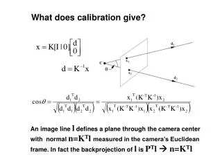
What does calibration give?. An image line l defines a plane through the camera center with normal n=K T l measured in the camera’s Euclidean frame. In fact the backprojection of l is P T l n= K T l. The image of the absolute conic.

What does calibration give?
E N D
Presentation Transcript
What does calibration give? An image line l defines a plane through the camera center with normal n=KTl measured in the camera’s Euclidean frame. In fact the backprojection of l is PTl n=KTl
The image of the absolute conic mapping between p∞ to an image is given by the planar homogaphy x=Hd, with H=KR absolute conic (IAC), represented by I3 withinp∞ (w=0) its image (IAC) • IAC depends only on intrinsics • angle between two rays • DIAC=w*=KKT • w K (Cholesky factorization) • image of circular points belong to w (image of absolute conic)
A simple calibration device • compute Hi for each square • (corners (0,0),(1,0),(0,1),(1,1)) • compute the imaged circular points Hi [1,±i,0]T • fit a conic w to 6 imaged circular points • compute K from w=K-T K-1 through Cholesky factorization (= Zhang’s calibration method)
Two-view geometry Epipolar geometry F-matrix comp. 3D reconstruction Structure comp.
Three questions: • Correspondence geometry: Given an image point x in the first view, how does this constrain the position of the corresponding point x’ in the second image? • (ii) Camera geometry (motion): Given a set of corresponding image points {xi ↔x’i}, i=1,…,n, what are the cameras P and P’ for the two views? • (iii) Scene geometry (structure): Given corresponding image points xi ↔x’i and cameras P, P’, what is the position of (their pre-image) X in space?
The epipolar geometry C,C’,x,x’ and X are coplanar
The epipolar geometry What if only C,C’,x are known?
The epipolar geometry All points on p project on l and l’
The epipolar geometry Family of planes p and lines l and l’ Intersection in e and e’
The epipolar geometry epipoles e,e’ = intersection of baseline with image plane = projection of projection center in other image = vanishing point of camera motion direction an epipolar plane = plane containing baseline (1-D family) an epipolar line = intersection of epipolar plane with image (always come in corresponding pairs)
The fundamental matrix F algebraic representation of epipolar geometry we will see that mapping is (singular) correlation (i.e. projective mapping from points to lines) represented by the fundamental matrix F
The fundamental matrix F algebraic derivation e’ is the image of C taken by the second camera
The fundamental matrix F correspondence condition The fundamental matrix satisfies the condition that for any pair of corresponding points x↔x’ in the two images
The fundamental matrix F F is the unique 3x3 rank 2 matrix that satisfies x’TFx=0 for all x↔x’ • Transpose: if F is fundamental matrix for (P,P’), then FT is fundamental matrix for (P’,P) • Epipolar lines: l’=Fx & l=FTx’ • Epipoles: on all epipolar lines, thus e’TFx=0, x e’TF=0, similarly Fe=0; • e’ is left null space of F • F has 7 d.o.f. , i.e. 3x3-1(homogeneous)-1(rank2) • F is a correlation, projective mapping from a point x to a line l’=Fx (not a proper correlation, i.e. not invertible)
Projective transformation and invariance Derivation based purely on projective concepts F invariant to transformations of projective 3-space unique not unique canonical form
~ ~ Show that if F is same for (P,P’) and (P,P’), there exists a projective transformation H so that P=HP and P’=HP’ ~ ~ Projective ambiguity of cameras given F previous slide: at least projective ambiguity this slide: not more! lemma: (22-15=7, ok)
F matrix, S skew-symmetric matrix (fund.matrix=F) Possible choice: Canonical representation: Canonical cameras given F F matrix corresponds to P,P’ iff P’TFP is skew-symmetric
PROJECTIVE RECONSTRUCTION Computation of F1i Ransac: - 8 point correspondence samples Computation of canonical cameras from F1i Triangulation of points in 3D • -Compute viewing rays from cameras • Intersect viewing rays associated to • corresponding points
The essential matrix ~fundamental matrix for calibrated cameras (remove K) 5 d.o.f. (3 for R; 2 for t up to scale) E is essential matrix if and only if two singularvalues are equal (and third=0) SVD
Motion from E Given Four solutions and
Four possible reconstructions from E (only one solution where points is in front of both cameras)
Motivation • Avoid explicit calibration procedure • Complex procedure • Need for calibration object • Need to maintain calibration
Motivation • Allow flexible acquisition • No prior calibration necessary • Possibility to vary intrinsics • Use archive footage
Constraints ? • Scene constraints • Parallellism, vanishing points, horizon, ... • Distances, positions, angles, ... Unknown scene no constraints • Camera extrinsics constraints • Pose, orientation, ... Unknown camera motion no constraints • Camera intrinsics constraints • Focal length, principal point, aspect ratio & skew Perspective camera model too general some constraints
Constraints on intrinsic parameters Constant e.g. fixed camera: Known e.g. rectangular pixels: square pixels: principal point known:
Self-calibration Upgrade from projective structure to metric structure using constraintsonintrinsic camera parameters • Constant intrinsics • Some known intrinsics, others varying • Constraints on intrincs and restricted motion (e.g. pure translation, pure rotation, planar motion) (Moons et al.´94, Hartley ´94, Armstrong ECCV´96) (Faugeras et al. ECCV´92, Hartley´93, Triggs´97, Pollefeys et al. PAMI´98, ...) (Heyden&Astrom CVPR´97, Pollefeys et al. ICCV´98,...)
A counting argument • To go from projective (15DOF) to metric (7DOF) at least 8 constraints are needed • Minimal sequence length should satisfy • Independent of algorithm • Assumes general motion (i.e. not critical)
rectangular pixels square pixels known internal parameters
Same camera for all images same intrinsics same image of the absolute conic e.g. moving cameras given sufficient images there is in general only one conic that projects to the same image in all images, i.e. the absolute conic This approach is called self-calibration, see later transfer of IAC:
Compute F from xi↔x‘i • Compute P,P‘ from F • Triangulate Xi from xi↔x‘i Obtain projective reconstruction (P,P‘,{Xi}) e.g.
The metric reconstruction will be t=0 Let the unknown plane at the infinity in the starting projective reconstruction be From
and Therefore, thus
Now Therefore, since Self-calibration equation and 8 unknowns:
Equations come from constraints on intrinsics: • known parameters (e.g. s=0 or square pixels) • fixed parameters (e.g. s, or aspect ratio) needed views: n, with Solution: nonlinear algorithms (Cipolla)
Uncalibrated visual odometry for ground plane motion (joint work with Simone Gasparini)
Problem formulation • Given: • an uncalibratedcamera mounted on a robot • the camera is fixed and aims at the floor • the robot moving on a planar floor (ground plane) • Determine: • the estimate of robot motion from observed features on the floor
Technique involved • Estimate the ground plane transformation (homography) between images taken before and after robot displacement
Motivations • Dead reckoning techniques are not reliable and diverge after few steps [Borenstein96] • Visual odometry techniques exploits cameras to recover motion • We use a single uncalibrated camera • 3D reconstruction with uncalibrated camera usually require auto-calibration • Non-planar motion is required [Triggs98] • Planar motion with different camera attitudes [Knight03] • Special devices is required (e.g. PTZ cameras) • Stereo cameras approaches [Nister04, Takaoka04, Agrawal06, Cheng06] • Catadioptric cameras approaches [Bunschoten03, Corke04] • Assume Single View Point (difficult setup) • Our method similar in spirit to [Wang05] and [Benhimane06] • We do not assume camera calibration
Problem formulation • Fixed uncalibrated camera mounted on a robot • The pose of the camera w.r.t. the robot is unknown • The projective transformation between ground plane and image plane is a homography T (3x3) • T does not change with robot motion • T is uknown