Download
1 / 66
660 likes | 785 Vues
Measuring the US Economy. Economic Indicators. Understanding the Lingo. Annualized Rates Example: GDP Q3 (Final) = $11,814.9B (5.5%) Q2: GDP = $2,914.38 B X 4 = $11,657.5 B Q3: GDP = $2,953.73 B X 4 = $11,814.9 B ($11,814.9 - $11,657.5) X 100 = 1.35% X4 = 5.5% $11,657.5.

E N D
Measuring the US Economy Economic Indicators
Understanding the Lingo • Annualized Rates Example: GDP Q3 (Final) = $11,814.9B (5.5%) Q2: GDP = $2,914.38 B X 4 = $11,657.5 B Q3: GDP = $2,953.73 B X 4 = $11,814.9 B ($11,814.9 - $11,657.5) X 100 = 1.35% X4 = 5.5% $11,657.5
Understanding the Lingo • Annualized Rates Supposed that prices increased by .3% during the month of November. The annualized inflation rate is .3%X12 = 3.6%
Understanding the Lingo • Nominal (Current) Dollars vs. Real (Constant) Dollars Example: GDP(Q2) = $11,657.5 GDP(Q3) = $11,814.9T (5.5%) CPI(Q2) = 111.2 CPI(Q3) = 112.4 (4.3%) Real GDP(Q2) = (11,657.5/111.2)*100 = $10,483.36 Real GDP(Q3) = (11,814.9/112.4)*100 = $10,511.47 ($10,511.47 - $10,483.36) X100 X 4 = 1.07% $10,483.36
Understanding the Lingo • Seasonally Adjusted
Understanding the Lingo • The X12 method estimates changes that occur in the same month each year and are generally of the same magnitude/direction. This seasonal component is then subtracted out.
Understanding the Lingo • Moving Averages Example: Consider the following monthly Inflation Statistics (Monthly % Changes)
Understanding the Lingo • Moving Averages A moving average takes out the volatility by averaging several observations. For example, a MA(3) would average the current observation with the previous 2 observations.
Understanding the Lingo • Revisions ALL ECONOMIC DATA IS CONSTANTLY BEING REVISED!!! Example: GDP is reported three times Q3(Advance): 3.7% Q3 (Preliminary): 3.9% Q3 (Final): 4.0%
Understanding the Lingo • Consensus Forecasts Most of the news services construct consensus surveys by polling economists for their predictions on key indicators
Understanding the Lingo • Benchmarking Some indicators are reported relative to some benchmark. Example: Consumer Confidence in December was 102.3 (1985 = 100) Example: The CPI in November was 191.0 (1982-1984 = 100)
Understanding the Lingo • The Business Cycle Since WWII, the US has experienced 10 Business cycles with the average recession lasting 10 months. The most recent cycle was 2001: • Peak (March 2001) • Trough (November 2001)
So Many Statistics….So Little Time! • The government releases over 50 statistics per month/quarter!! They can be roughly divided into 5 categories • Consumer Sector • Business Sector • Public Sector • International • Prices
Major Indicators • Consumer Sector (70% of Economic Activity) • Retail Sales (Census Bureau) • Consumer Credit (Federal Reserve) • Personal Income and Spending (BEA) • Employment Report (BLS) • New Claims For Unemployment Insurance (Dept of Labor) • Consumer Confidence/Sentiment (Conference Board/U. of Michigan) • Auto Sales (Dept. of Commerce)
Major Indicators • Business Sector(17% of Economic Activity) • Industrial Production (Federal Reserve) • Capacity Utilization (Federal Reserve) • ISM Index (Institute for Supply Management) • Durable Goods Orders (Census Bureau) • Factory Orders (Census Bureau) • Housing Starts (Census Bureau) • New/Existing Home Sales (Nat. Assoc. of Realtors/Census Bureau) • MBA Mortgage Applications (Mortgage Bankers Assoc.) • Business inventories (Census Bureau)
Major Indicators • Public Sector(19% of Economic Activity) • Construction Spending (Census) • Federal Budget Report (Treasury Dept) • International Sector (-6% of Economic Activity) • Net Exports (Bureau of Economic Analysis) • Current Account (Bureau of Economic Analysis)
Major Indicators • Prices • Consumer Price Index (BLS) • Producer Price Index (BLS) • Employment Cost Index (BLS) • Non-Farm Productivity (BLS) • Import/Export Prices (BLS)
Criteria For “Good” Indicators • Accuracy: • Most economic data is compiled through surveys – larger survey pools are more accurate. • To measure consumer confidence, the conference board polls 5,000 households per month. • To measure prices, the bureau of labor statistics polls 28,000 retail outlets per month! (on 80,000 products) • Some statistics are subject to large revisions. • Housing starts are rarely revised while the monthly construction spending report often gets substantial revisions
Criteria For “Good” Indicators • Timeliness The BLS employment situation report comes out a week after the end of the month, while consumer credit is reported on a two month delay.
Predictive Ability • Blue Arrow = Peak • Red Arrow = Trough
Predictive Ability • Blue Arrow = Peak • Red Arrow = Trough
Predictive Ability • Blue Arrow = Peak • Red Arrow = Trough
Criteria For “Good” Indicators • Business Cycle Stage • During recessions, we’re looking for signs of recovery • Housing Starts • Auto Sales • Employment • During expansions we tend to be more concerned with inflation • CPI • Employment cost index
Criteria For “Good” Indicators • Who Are You? • Stock markets are most concerned with consumer/business spending which drive corporate profits (Employment, Retail Sales) • Bond Markets worry about inflation (CPI, PPI) • Foreign Exchange Markets (Current Account, GDP, Productivity)
A Shortcut • Index of Leading Indicators (Conference Board) • Average Hourly Workweek in Manufacturing (19.7%) • Weekly Unemployment Claims (2.5%) • Manufacturers’ New Orders – Consumer Goods (5.9%) • Manufacturers’ New Orders – Capital Goods (1.5%) • Vendor Performance (Delivery Time Index) (2.9%) • Building Permits for New Homes (2%) • Index of Consumer Expectations (1.9%) • S&P Index (2.9%) • Real (inflation adjusted) M2 Money Supply (27.7%) • Interest Spread Between 10 Yr. Bonds & Fed Funds Rate (33%)
Index of Leading Indicators • Blue Arrow = Peak • Red Arrow = Trough
The Big One: Employment What is it: Total (Non-Farm) Employment, Unemployment Rate, Average Duration, etc…..Are people working? Release Time: 8:00AM, the first Friday of the month following the coverage month Frequency: Monthly Source: Bureau of Labor Statistics Revisions: Frequent Revisions…sometimes major!
The Household Survey • Each month, the BLS contacts 60,000 households (95% response rate) and places each in one of four categories: • Under 16 or institutionalized (or military) • Choose not to work: Not in Labor Force • Choose to work and are working: Employed • Choose to work, but can’t find a job: Unemployed Unemployment Rate = D/(D+C)
US Population: 290M Civilian Population: 220M Labor Force: 147M Employment: 139M Unemployment: 8M Participation Rate (147M/220M)*100 = 66% Employment Ratio (138M/220M)*100 = 62% Unemployment Rate (8M/147M)*100 = 5.4% UR = 1 – (ER/PR) Household Survey
Establishment (Payroll) Survey • Each month, the BLS contacts 400,000 firms!! (60% - 70%) response rate. Each firm is asked to report total employment. • Employment: 131M??
The US Labor Market • Labor markets are difficult to characterize because they are always in motion….. EMPLOYED NOT IN LABOR FORCE UNEMPLOYED Average Turnover is around 2.5 Million people per Month!!
Most unemployment spells in the US are short. <5 Wks: 2.9m 5-15 Wks: 2.2m + >15 Wks: 2.9m Total: 8.0m Average duration in the US is approx. 19wks Median: 9wks Average Duration In 1 year, how many people are unemployed for 5 wks? (52/5)*2.9M = 30.1M How many people are unemployed for 10 wks? (52/10)*2.2M = 11.4M For 20 wks? +(52/20)*2.9M = 7.5M Total 49M AD = (30.1/49)*(5wks) + (11.4/49)*(10wks) + (7.5/49)*(20wks) =8.5wks Duration
What’s “Normal” in the Labor Market? Frictional Unemployment: Currently unemployed, but in the process of getting a job (i.e., short term unemployment): 3.5% + Structural Unemployment (chronic unemployment): 1.5% “Natural Rate of Unemployment”: 5% • Given the current unemployment rate of 5.4%, we currently have a cyclical unemployment rateof .4%
The cost of unemployment • “Capacity Output” of an economy is the level of output associated with full employment (i.e., unemployment is at the natural rate) • The “output gap” is the difference between capacity output and actual output • Okun’s law states that every 1% increase in cyclical unemployment increases the output gap by 2.5%. • Therefore, our current .4% cyclical unemployment rate implies an output gap of 1% GPD ( Roughly $110B! )
GDP (Gross Domestic Product) What is it: Current dollar value of all goods and service produced in the US Release Time: 8:30AM, The final week of the month following the covered quarter (each quarter has three estimates: Advance, Preliminary, Final) Frequency: Quarterly Source: Bureau of Economic Analysis Revisions: They usually get it right by the final revision.
Calculating GDP • If our economy was horizontally oriented (i.e. everyone produces final goods) economy, calculating GDP would be easy: GDP = Price*Quantity (Added up over all goods) • Our economy is vertically oriented (some manufacturers produce intermediate goods). Therefore, we must avoid double counting. • Each manufacturer reports output on a value added basis
GDP (2003) Consumer Goods: $7,752.2B Investment Goods: $1,667.5B Government Expenditures: $2,055.7B Net Exports: -$491.5B $10,983.9 Income (2003) GDP: $10,983.9 - Net Factor Payments: $37.9 GNP: $10,946.0 Depreciation $1,370.1 NNP: $9,575.9 Indirect Taxes: $834.4 National Income: $8741.5 National Income and Product Accounts
Income (2003) GDP: $10,983.9 - Net Factor Payments: $37.9 GNP: $10,946.0 Depreciation $1,370.1 NNP: $9,575.9 Indirect Taxes: $834.4 National Income: $8741.5 Income (2003) Wages: $6,039.5 Proprietor’s Income: $774.6 Rental Income: $127.9 Corporate Profits: $1,294.2 Interest: $546.9 National Income: $8,783.1 Statistical Discrepancy: 41.6B National Income and Product Accounts
Real vs. Nominal • Recall that GDP will grow either because we are producing more, or because prices are increasing. To correct for this, the BEA, repeats the previous calculations using a set of “Base year” prices. GDP (2003 Prices) = $10,983.9 GDP (2000 Prices) = $10,397.2 Note that this implicitly implies a Price index……The GDP Deflator! P(2000) = 1 P(2003) = $10,983.9/$10,397.2 = 1.056 (i.e. prices increased by 5.6% from 2000 – 2003)
GDP Facts • GDP in 2004 is $11,649.3 Billion while GDP in 1950 was $275.7 Billion. (an increase of 4200%). • Real GDP (2000 $s) in 2004 was $10,788.9 Billion while Real GDP in 1950 was $1,777.5 Billion (A 600% increase) • Real GDP per capita in 2003 is $36,911 compared to $10,736 in 1950 ( a 350% increase). • Median real income in 2003 is approximately $24,000 while median real income in 1950 was approximately $8,000 (a 300% increase)
CPI (Consumer Price Index) What is it: The “Average” Price of Consumer Goods in the US Release Time: 8:30AM, The second or third week following the covered month Frequency: Monthly Source: Bureau of Labor Statistics Revisions: No Revisions except for an annual correction done in February.
Fixed Weight Indices • A price index is meant to capture the average price of goods and services in the economy. Therefore, any price index should be a weighted average of all (or at least, most) prices in the economy. • With any fixed weight index, the weights used in the index are chosen ex ante and remain fixed over time (hence, the name fixed weight index). • Think of the a fixed weight index as simply defining a “basket” of goods. The value of that index is the cost of that basket.