Binary Heaps in Data Structures: Lecture Summary
Learn about binary heaps, their structure properties, array implementation, and operations like FindMin, DeleteMin, and Insert in this detailed lecture summary. Discover the efficiency of binary heaps in quickly finding priority items.

Binary Heaps in Data Structures: Lecture Summary
E N D
Presentation Transcript
Binary Heaps CSE 373 Data Structures Lecture 11
Readings • Reading • Sections 6.1-6.4 Binary Heaps - Lecture 11
Revisiting FindMin • Application: Find the smallest ( or highest priority) item quickly • Operating system needs to schedule jobs according to priority instead of FIFO • Event simulation (bank customers arriving and departing, ordered according to when the event happened) • Find student with highest grade, employee with highest salary etc. Binary Heaps - Lecture 11
Priority Queue ADT • Priority Queue can efficiently do: • FindMin (and DeleteMin) • Insert • What if we use… • Lists: If sorted, what is the run time for Insert and FindMin? Unsorted? • Binary Search Trees: What is the run time for Insert and FindMin? • Hash Tables: What is the run time for Insert and FindMin? Binary Heaps - Lecture 11
Less flexibility More speed • Lists • If sorted: FindMin is O(1) but Insert is O(N) • If not sorted: Insert is O(1) but FindMin is O(N) • Balanced Binary Search Trees (BSTs) • Insert is O(log N) and FindMin is O(log N) • Hash Tables • Insert O(1) but no hope for FindMin • BSTs look good but… • BSTs are efficient for all Finds, not just FindMin • We only need FindMin Binary Heaps - Lecture 11
Better than a speeding BST • We can do better than Balanced Binary Search Trees? • Very limited requirements: Insert, FindMin, DeleteMin. The goals are: • FindMin is O(1) • Insert is O(log N) • DeleteMin is O(log N) Binary Heaps - Lecture 11
Binary Heaps • A binary heap is a binary tree (NOT a BST) that is: • Complete: the tree is completely filled except possibly the bottom level, which is filled from left to right • Satisfies the heap order property • every node is less than or equal to its children • or every node is greater than or equal to its children • The root node is always the smallest node • or the largest, depending on the heap order Binary Heaps - Lecture 11
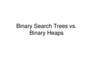
Heap order property • A heap provides limited ordering information • Each path is sorted, but the subtrees are not sorted relative to each other • A binary heap is NOT a binary search tree -1 2 1 1 0 6 4 6 2 0 7 5 8 4 7 These are all valid binary heaps (minimum) Binary Heaps - Lecture 11
Binary Heap vs Binary Search Tree Binary Heap Binary Search Tree min value 5 94 10 94 10 97 min value 97 24 5 24 Parent is less than both left and right children Parent is greater than left child, less than right child Binary Heaps - Lecture 11
Structure property • A binary heap is a complete tree • All nodes are in use except for possibly the right end of the bottom row Binary Heaps - Lecture 11
Examples 6 2 4 2 4 6 complete tree, heap order is "max" 5 not complete 2 2 4 6 5 6 7 5 7 4 complete tree, heap order is "min" complete tree, but min heap order is broken Binary Heaps - Lecture 11
Array Implementation of Heaps (Implicit Pointers) • Root node = A[1] • Children of A[i] = A[2i], A[2i + 1] • Keep track of current size N (number of nodes) 1 2 2 3 - 2 4 6 7 5 4 6 value index 0 1 2 3 4 5 6 7 7 5 4 5 N = 5 Binary Heaps - Lecture 11
FindMin and DeleteMin • FindMin: Easy! • Return root value A[1] • Run time = ? • DeleteMin: • Delete (and return) value at root node 2 4 3 7 5 8 10 11 9 6 14 Binary Heaps - Lecture 11
DeleteMin • Delete (and return) value at root node 4 3 7 5 8 10 11 9 6 14 Binary Heaps - Lecture 11
Maintain the Structure Property • We now have a “Hole” at the root • Need to fill the hole with another value • When we get done, the tree will have one less node and must still be complete 4 3 7 5 8 10 11 9 6 14 4 3 7 5 8 10 11 9 6 14 Binary Heaps - Lecture 11
Maintain the Heap Property • The last value has lost its node • we need to find a new place for it • We can do a simple insertion sort operation to find the correct place for it in the tree 14 4 3 7 5 8 10 11 9 6 Binary Heaps - Lecture 11
DeleteMin: Percolate Down 14 ? 14 3 3 ? 4 8 4 3 4 7 5 14 10 7 5 8 10 7 5 8 10 11 9 6 11 9 6 11 9 6 • Keep comparing with children A[2i] and A[2i + 1] • Copy smaller child up and go down one level • Done if both children are item or reached a leaf node • What is the run time? Binary Heaps - Lecture 11
Percolate Down PercDown(i:integer, x :integer): { // N is the number of entries in heap// j : integer; Case{ 2i > N : A[i] := x; //at bottom// 2i = N : if A[2i] < x then A[i] := A[2i]; A[2i] := x; else A[i] := x; 2i < N : if A[2i] < A[2i+1] then j := 2i; else j := 2i+1; if A[j] < x then A[i] := A[j]; PercDown(j,x); else A[i] := x; }} Binary Heaps - Lecture 11
DeleteMin: Run Time Analysis • Run time is O(depth of heap) • A heap is a complete binary tree • Depth of a complete binary tree of N nodes? • depth = log2(N) • Run time of DeleteMin is O(log N) Binary Heaps - Lecture 11
Insert • Add a value to the tree • Structure and heap order properties must still be correct when we are done 2 3 4 8 7 5 14 10 11 9 6 Binary Heaps - Lecture 11
Maintain the Structure Property • The only valid place for a new node in a complete tree is at the end of the array • We need to decide on the correct value for the new node, and adjust the heap accordingly 2 3 4 8 7 5 14 10 11 9 6 Binary Heaps - Lecture 11
Maintain the Heap Property • The new value goes where? • We can do a simple insertion sort operation to find the correct place for it in the tree 3 4 8 7 5 14 10 11 9 6 2 Binary Heaps - Lecture 11
Insert: Percolate Up 2 3 ? 3 3 4 8 4 8 8 7 5 14 10 7 14 10 7 4 14 10 ? ? 11 9 6 11 9 6 11 9 6 5 5 2 2 • Start at last node and keep comparing with parent A[i/2] • If parent larger, copy parent down and go up one level • Done if parent item or reached top node A[1] • Run time? Binary Heaps - Lecture 11
Insert: Done 2 3 8 7 4 14 10 11 9 6 5 • Run time? Binary Heaps - Lecture 11
PercUp • Define PercUp which percolates new entry to correct spot. • Note: the parent of i is i/2 PercUp(i : integer, x : integer): { ???? } Binary Heaps - Lecture 11
Sentinel Values - • Every iteration of Insert needs to test: • if it has reached the top node A[1] • if parent item • Can avoid first test if A[0] contains a very large negative value • sentinel - < item, for all items • Second test alone always stops at top 2 3 8 7 4 10 9 11 9 6 5 - 2 3 8 7 4 10 9 11 9 6 5 value index 8 9 10 11 12 13 0 1 2 3 4 5 6 7 Binary Heaps - Lecture 11
Binary Heap Analysis • Space needed for heap of N nodes: O(MaxN) • An array of size MaxN, plus a variable to store the size N, plus an array slot to hold the sentinel • Time • FindMin: O(1) • DeleteMin and Insert: O(log N) • BuildHeap from N inputs : O(N) Binary Heaps - Lecture 11
Build Heap BuildHeap { for i = N/2 to 1 by –1 PercDown(i,A[i]) } 1 N=11 11 11 2 3 5 10 5 10 4 5 6 7 9 4 8 12 9 3 8 12 2 7 6 3 2 7 6 4 8 11 9 10 Binary Heaps - Lecture 11
Build Heap 11 11 5 10 5 8 2 3 8 9 2 3 10 12 9 7 6 4 9 7 6 4 Binary Heaps - Lecture 11
Build Heap 11 2 2 8 3 8 5 3 10 12 5 4 10 12 9 7 6 4 9 7 6 11 Binary Heaps - Lecture 11
Analysis of Build Heap • Assume N = 2K –1 • Level 1: k -1 steps for 1 item • Level 2: k - 2 steps for 2 items • Level 3: k - 3 steps for 4 items • Level i : k - i steps for 2i-1 items Binary Heaps - Lecture 11
Other Heap Operations • Find(X, H): Find the element X in heap H of N elements • What is the running time? O(N) • FindMax(H): Find the maximum element in H • Where FindMin is O(1) • What is the running time? O(N) • We sacrificed performance of these operations in order to get O(1) performance for FindMin Binary Heaps - Lecture 11
Other Heap Operations • DecreaseKey(P,,H): Decrease the key value of node at position P by a positive amount , e.g., to increase priority • First, subtract from current value at P • Heap order property may be violated • so percolate up to fix • Running Time: O(log N) Binary Heaps - Lecture 11
Other Heap Operations • IncreaseKey(P,,H): Increase the key value of node at position P by a positive amount , e.g., to decrease priority • First, add to current value at P • Heap order property may be violated • so percolate down to fix • Running Time: O(log N) Binary Heaps - Lecture 11
Other Heap Operations • Delete(P,H): E.g. Delete a job waiting in queue that has been preemptively terminated by user • Use DecreaseKey(P,,H) followed by DeleteMin • Running Time: O(log N) Binary Heaps - Lecture 11
Other Heap Operations • Merge(H1,H2): Merge two heaps H1 and H2 of size O(N). H1 and H2 are stored in two arrays. • Can do O(N) Insert operations: O(N log N) time • Better: Copy H2 at the end of H1 and use BuildHeap. Running Time: O(N) Binary Heaps - Lecture 11
PercUp Solution PercUp(i : integer, x : integer): { if i = 1 then A[1] := x else if A[i/2] < x then A[i] := x; else A[i] := A[i/2]; Percup(i/2,x); } Binary Heaps - Lecture 11