Dynamic Sets and Searching

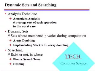
1. Dynamic Sets and Searching Analysis Technique Amortized Analysis// average cost of each operation in the worst case Dynamic Sets// Sets whose membership varies during computation Array Doubling Implementing Stack with array doubling Searching// Exist or not, in where Binary Search Trees Hashing

2. Amortized Analysis • Provides average cost of each operation in the worst case for successive operations • Aggregate method • show for a sequence of n operations takes worst-case time T(n) in total • In the worst case, the average cost, or amortized cost, per operation is therefore T(n)/n • Accounting method // spreading a large cost over time • amortized cost = actual cost + accounting cost • assign different accounting cost to different operations • 1. the sum of accounting costs is nonnegative for any legal sequence of operations • 2. to make sure it is feasible to analyze the amortized cost of each operation

3. Array Doubling • We don’t know how big an array we might need when the computation begins • If not more room for inserting new elements, • allocating a new array that is twice as large as the current array • transferring all the elements into the new array • Let t be the cost of transferring one element • suppose inserting the (n+1) element triggers an array-doubling • cost t*n for this array-doubling operation • cost t*n/2 + t*n/4 + t*n/8 + … for previous array-doubling, i.e. cost less than t*n • total cost less than 2t*n • The average cost for each insert operation = 2t

4. Implementing Stack with array doubling • Array doubling is used behind the scenes to enlarge the array as necessary • Assuming actual cost of push or pop is 1 • when no enlarging of the array occurs • the actual cost of push is 1 + t*n • when array doubling is required • Accounting scheme, assigning • accounting cost for a push to be 2t • when no enlarging of array occurs • accounting cost for push to be –t*n + 2t • when array doubling is required • The amortized cost of each push operation is 1+2t • From the time the stack is created, the sum of the accounting cost must never be negative.

5. Searching: Binary Search Trees • Binary Search Tree property • A binary tree in which the nodes have keys from an ordered set has the binary search tree property • if the key at each node is greater than all the keys in its left subtree and • less than or equal to all keys in its right subtree • In this case the binary tree is called a binary search tree • An inorder traversal of a binary search tree produces a sorted list of keys.

6. Binary Search Trees, e.g. • Binary Search trees with different degrees of balances • Black dots denote empty trees

7. Binary Search Tree Retrieval • Element bstSearch(BinTree bst, Key K) • Element found • if (bst == nil) • found = null; • else • Element root = root(bst); • If (K == root.key) • found = root; • else if (K < root.key) • found = bstSearch (leftSubtree(bst), K); • else • found = bstSearch(rightSubtree(bst), K); • return found;

8. Analysis of Binary Search Tree Retrieval • use the number of internal nodes of the tree that are examined which searching for key • let it be n • For a long chain tree structure, (n) • For a tree as balanced as possible, (lg n) • >> The objective is to make the tree as balanced as possible • Technique: Binary Tree Rotations

9. Binary Tree Rotations • Left Rotation on (15, 25)

10. Making binary search treesas balanced as possible • Red-Black Tree • Let T be a red-black tree with n internal nodes. Then no node has depth greater than 2 lg(n + 1).

11. Hashing to aid searching • Imagine that we could assign a unique array index to every possible key that could occur in an application. • locating, inserting, deleting elements could be done very easily and quickly • key space is much too large • The purpose of hashing is to translate (by using hash function) an extremely large key space into a reasonable small range of integers (called hash code). • Hash Table • an array H on indexes (hash code) 0, …, h-1 • hash function maps a key into an integer in the range 0, …, h-1 • Each entry may contain one or more keys! • Hash function is a many-to-one function

12. Hash Table, e.g. • data k: 1055, 1492, 1776, 1812, 1918, and 1945 • hash function • hashCode(k) = 5k mod 8 • hashCode: key • 0: 1776 • 1: • 2: • 3: 1055 • 4: 1492, 1812 // Collision! • 5: 1945 • 6: 1918 • 7:

13. Handling Collisions: Closed Address Hashing • H[i] is a linked list • hashCode: key • 0: -> 1776 • 1: -> • 2: -> • 3: ->1055 • 4: ->1492 -> 1812 • 5: ->1945 • 6: ->1918 • 7: -> • To search a given key K, first compute its hash code, say i, then search through the linked list at H[i], comparing K with the keys of the elements in the list.

14. Analysis of Closed Address Hashing • Searching for a key • Basic Operation: comparisons • Assume computing a hash code equals aunits of comparisons • there are total n elements stored in the table, • each elements is equally likely to be search • Average number of comparison for an unsuccessful search (after hashing) equal • Au(n) = n/h • Average cost of a successful search • when key i = 1, …, n, was inserted at the end of a linked list, each linked list had average length given by (i – 1)/h • expected number of key comparisons = 1 + comparisons make for inserting an element at the end of a linked list • As(n) = 1/n {i=1 to n}( 1 + (i - 1)/h ) = 1 + n/(2h) + 1/(2h)

15. Assuming uniformly distribution of hash code • hash code for each key in our set is equally likely to be any integer in the range 0, …, h-1 • If n/h is a constants then • O(1) key comparisons can be achieved, on average, for successful search and unsuccessful search. • Uniformly distribution of hash code depends on the choice of Hash Function

16. Choosing a Hash Function • // for achieve uniformly distribution of hash code • If the key type is integer • hashCode(K) = (a K) mod h • Choose h as a power of 2, and h >= 8 • Choose a = 8 Floor[h/23] + 5 • If the key type is string of characters, treat them as sequence of integers, k1, k2, k3, …, kl • hashCode(K) = (al k1 + al-1k2 + …+a kl) mod h • Use array doubling whenever n/h (called load factor, where n is the number of elements in the table) gets high, say 0.5

17. Handling Collisions: Open Address Hashing • is a strategy for storing all elements in the array of the hash table, rather than using linked lists to accommodate collisions • if the hash cell corresponding to the hash code is occupied by a different elements, • then a sequence of alternative locations for the current element is defined (by rehashing) • Rehashing by linear probing • rehash(j) = (j+1) mod h • where j is the location most recently probed, • initially j = i, the hash code for K • Rehashing by double hashing • rehash(j, d) = (j + d) mod h • e.g. d = hashIncr(K) = (2K + 1) mod h • // computing an odd increment ensures that whole hash table is accessed in the search (provided h is a power of 2)

18. Open Address Hashing, e.g. Linear probing • hashCode: key • 0: 1776 • 1: • 2: • 3: 1055 • 4: 1492 • 5: 1945 • 6: 1918 • 7: • Now insert 1812, hashcode(1812) = 4, i.e. i = 4 • h = 8, initially j = i = 4 • rehash(j) = (j+1) mod h • rehash(4) = (4+1) mod 8 = 5 // collision again • rehash(5) = (5+1) mod 8 = 6 // collision again • … put in 7

19. Retrieval and Deletion under open addressing hashing • Retrieval procedure imitates the insertion procedure, stop search as soon as emptyCell is encountered. • Deletion of a key • cannot simply delete the the key and assign the cell to emptyCell // cause problem for retrieval procedure • need to assign the cell to a value indicating “obsolete”