Exam #2 Results
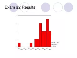
Exam #2 Results. Exam #2 Results. Exam #2 Results. All t-scores refer to Repeated-Measures t-tests For the exam as a whole: t (30) = 3.31, p = .002, d = 1.21 Cohen’s conventions for d : .2 = small, .5 = medium, .8 = large. One-Way Analysis of Variance (ANOVA). One-Way ANOVA.

Exam #2 Results
E N D
Presentation Transcript
Exam #2 Results • All t-scores refer to Repeated-Measures t-tests • For the exam as a whole: • t(30) = 3.31, p = .002, d = 1.21 • Cohen’s conventions for d: .2 = small, .5 = medium, .8 = large
One-Way ANOVA • One-Way Analysis of Variance • aka One-Way ANOVA • Most widely used statistical technique in all of statistics • One-Way refers to the fact that only one IV and one DV are being analyzed (like the t-test) • i.e. An independent-samples t-test with treatment and control groups where the treatment (present in the Tx grp and absent in the control grp) is the IV
One-Way ANOVA • Unlike the t-test, the ANOVA can look at levels or subgroups of IV’s • The t-test can only test if an IV is there or not, not differences between subgroups of the IV • I.e. our experiment is to test the effect of hair color (our IV) on intelligence • One t-test can only test if brunettes are smarter than blondes, any other comparison would involve doing another t-test • A one-way ANOVA can test many subgroups or levels of our IV “hair color”, for instance blondes, brunettes, and redheads are all subtypes of hair color, can so can be tested with one one-way ANOVA
One-Way ANOVA • Other examples of subgroups: • If “race” is your IV, then caucasian, african-american, asian-american, hispanic, etc. are all subgroups/levels • If “gender” is your IV, than male and female are you levels • If “treatment” is your IV, then some treatment, a little treatment, and a lot of treatment can be your levels
One-Way ANOVA • OK, so why not just do a lot of t-tests and keep things simple? • Many t-tests will inflate our Type I Error rate! • This is an example of using many statistical tests to evaluate one hypothesis – see: the Bonferroni Correction • It is less time consuming • There is a simple way to do the same thing in ANOVA, they are called post-hoc tests, and we will go over them later on • However, with only one DV and one IV (with only two levels), the ANOVA and t-test are mathematically identical, since they are essentially derived from the same source
One-Way ANOVA • Therefore, the ANOVA and the t-test have similar assumptions: • Assumption of Normality • Like the t-test you can place fast and loose with this one, especially with large enough sample size – see: the Central Limit Theorem • Assumption of Homogeneity of Variance • Like the t-test this isn’t problematic unless one level’s variance is much larger than one the others (~4 times as large) – the one-way ANOVA is robust to small violations of this assumption, so long as group size is roughly equal
One-Way ANOVA • Independence of Observations • Like the t-test, the ANOVA is very sensitive to violations of this assumption – if violated it is more appropriate to use a Repeated-Measures ANOVA • The basic logic behind the ANOVA: • The ANOVA yields and F-statistic (just like the t-test gave us a t-statistic) • The basic form of the F-statistic is: MSgroups/MSerror
One-Way ANOVA • The basic logic behind the ANOVA: • MS = mean square or the mean of squares (why it is called this will be more obvious later) • MSbetween or MSgroups = average variability (variance) between the levels of our IV/groups • Ideally we want to maximize MSgroups, because we’re predicting that our IV will differentially effect our groups • i.e. if our IV is treatment, and the levels are no treatment vs. a lot of treatment, we would expect the treatment group mean to be very different than the no treatment mean – this results in lots of variability between these groups
One-Way ANOVA • The basic logic behind the ANOVA: • MSwithin or MSerror = average variance among subjects in the same group • Ideally we want to minimize MSerror, because ideally our IV (treatment) influences everyone equally – everyone improves, and does so at the same rate (i.e. variability is low) • If F = MSgroups/MSerror, then making MSgroups large andMSerror small will result in a large value of F • Like t, a large value corresponds to small p-values, which makes it more likely to reject Ho
One-Way ANOVA • However, before we calculate MS, we need to calculate what are called sums of squares, or SS • SS = the sum of squared deviations around the mean • Does this sound familiar? What does this sound like? • Just like MS, we have SSerror and SSgroups • Unlike MS, we also have SStotal = SSerror + SSgroups
One-Way ANOVA • SStotal = Σ(Xij - )2 = • It’s the formula for our old friend variance, minus the n-1 denominator! • Note: N = the number of subjects in all of the groups added together
One-Way ANOVA • SSgroups = • This means we: • Subtract the grand mean, or the mean of all of the individual data points, from each group mean • Square these numbers • Multiply them by the number of subjects from that particular group • Sum them • Note: n = number of subjects per group • Hint: The number of numbers that you sum should equal the number of groups
One-Way ANOVA • That leaves us with SSerror = SStotal – SSgroups • Remember: SStotal = SSerror + SSgroups • Degrees of freedom: • Just as we have SStotal,SSerror, and SSgroups, we also have dftotal, dferror, and dfgroups • dftotal =N – 1 OR the total number of subjects in all groups minus 1 • dfgroups = k – 1 OR the number of levels of our IV (aka groups) minus 1 • dferror = N – k OR the total number of subjects minus the number of groups OR dftotal -dfgroups
One-Way ANOVA • Now that we have our SS and df, we can calculate MS • MSgroups = SSgroups/dfgroups • MSerror = SSerror/dferror • Remember: • MSbetween or MSgroups = average variability (variance) between the levels of our IV/groups • MSwithin or MSerror = average variance among subjects in the same group
One-Way ANOVA • We then use this to calculate our F-statistic: • F = MSgroups/MSerror • Then we compare this to the F-Table (Table E.3 and E.4, page 516 & 517 in your text) • There are actually two tables, one if you set your α = .05 (Table E.3, pg. 516), and one if your α = .01 (Table E.4, pg. 517)
One-Way ANOVA • “Degrees of Freedom for Numerator” = dfgroup • “Degrees of Freedom for Denominator” = dferror
One-Way ANOVA • This value = our critical F • Like the critical t, if our observed F is larger than the critical F, then we reject Ho • Hypothesis testing in ANOVA: • Since ANOVA tests for differences between means for multiple groups or levels of our IV, then H1 is that there is a difference somewhere between these group means • H1 = μ1 ≠ μ2 ≠ μ3 ≠ μ4, etc… • Ho = μ1 = μ2 = μ3 = μ4, etc…
One-Way ANOVA • However, our F-statistic does not tell us where this difference lies • If we have 4 groups, group 1 could differ from groups 2-4, groups 2 and 4 could differ from groups 1 and 3, group 1 and 2 could differ from 3, but not 4, etc. • Since our hypothesis should be as precise as possible (presuming you’re researching something that isn’t completely new), you will want to determine the precise nature of these differences • You can do this using multiple comparison techniques
One-Way ANOVA • But before we go into that, an example: • Example #1: • An experimenter wanted to examine how depth of processing material and age of the subjects affected recall of the material after a delay. One group consisted of Younger subjects who were presented the words to be recalled in a condition that elicited a Low level of processing. A second group consisted of Younger subjects who were given a task requiring the Highest level of processing. The two other groups were Older subjects who were given tasks requiring either Low or High levels of processing. The data follow: • Younger/Low 8 6 4 6 7 6 5 7 9 7 • Younger/High 21 19 17 15 22 16 22 22 18 21 • Older/Low 9 8 6 8 10 4 6 5 7 7 • Older/High 10 19 14 5 10 11 14 15 11 11
One-Way ANOVA • Example #1: • DV = memory performance, IV = age/depth of processing (4 levels) • H1: That at least one of the four groups will be different from the other three • μ1 ≠ μ2 ≠ μ3 ≠ μ4 • Ho: That none of the four groups will differ from one another • μ1 = μ2 = μ3 = μ4 • dftotal = 40-1 = 39; dfgroup = 4-1 = 3; dferror = 40-4 = 36 • Critical Fα=.05 = between 2.92 and 2.84 = (2.92+2.84)/2 = 2.88
One-Way ANOVA • Grand Mean = (65+193+70+110)/40 = 10.95 • MeanY/L = 65/10 = 6.5 • MeanY/H = 193/10 = 19.3 • MeanO/L = 70/10 = 7 • MeanO/H = 110/10 = 11
One-Way ANOVA • SStotal = • ΣX2=441 + 3789 + 520 +1386 = 6,136 • (ΣX)2= (65 +193+70+110)2= 191,844 • SStotal = 1,339.9
One-Way ANOVA • SSgroup = 1,051.3 • SSerror = SStotal – SSgroups = 1,339.9 – 1,051.3 = 288.6 • MSgroups = 1051.3/3 = 350.4333 • MSerror = 288.6/36 = 8.0166666 • F = 350.4333/8.0166= 43.71
One-Way ANOVA • Example #1: • Since our observed F > critical F, we would reject Ho and conclude that one of our four groups is significantly different from one of our other groups
One-Way ANOVA • Example #2: • What effect does smoking have on performance? Spilich, June, and Renner (1992) asked nonsmokers (NS), smokers who had delayed smoking for three hours (DS), and smokers who were actively smoking (AS) to perform a pattern recognition task in which they had to locate a target on a screen. The data follow:
One-Way ANOVA • Example #2: • Get into groups of 2 or more • Identify the IV, number of levels, and the DV • Identify H1 and Ho • Identify your dftotal, dfgroups, and dferror, and your critical F • Calculate your observed F • Would you reject Ho? State your conclusion in words.
One-Way ANOVA • Multiple Comparison Techniques: • The Bonferroni Method • You could always run 2-sample t-tests on all possible 2-group combinations of your groups, although with our 4 group example this is 6 different tests • Running 6 tests @ (α = .05) = (α = .3) • Running 6 tests @ (α = .05/6 = .083) = (α = .05) • This controls what is called the familywise error rate – in our previous example, all of the 6 tests that we run are considered a family of tests, and the familywise error rate is the α for all 6 tests combined – we want to keep this at .05
One-Way ANOVA • Multiple Comparison Techniques: • Fisher’s Least Significant Difference (LSD) Test • Test requires a significant F – although the Bonferroni method didn’t require a significant F, you shouldn’t use it unless you have one • Why would you look for a difference between two groups when your F said there isn’t one?
One-Way ANOVA • Multiple Comparison Techniques: • This is what is called statistical fishing and is very bad – you should not be conducting statistical tests willy-nilly without just cause or a theoretical reason for doing so • Think of someone fishing in a lake, you don’t know if anything is there, but you’ll keep trying until you find something – the idea is that if your hypothesis is true, you shouldn’t have to look to hard to find it, because if you look for anything hard enough you tend to find it
One-Way ANOVA • Multiple Comparison Techniques: • Fisher’s LSD • We replace in our 2-sample t-test formula with MSerror, and we get: • We then test this using a critical t, using our t-table and dferror as our df • You can use either a one-tailed or two-tailed test, depending on whether or not you think one mean is higher or lower (one-tailed) or possibly either (two-tailed) than the other
One-Way ANOVA • Multiple Comparison Techniques: • Fisher’s LSD • However, with more than 3 groups, using Fisher’s LSD results in an inflation of α (i.e. with 4 groups α = .1) • You could use the Bonferroni method to correct for this, but then why not just use it in the first place? • This is why Fisher’s LSD is no longer widely used and other methods are preferred
One-Way ANOVA • Multiple Comparison Techniques: 3. Tukey’s Honestly Significant Difference (HSD) test • Very popular, but too conservative in that it result in a low degree of Type I Error but too high Type II Error (incorrectly rejects H1) • Scheffe’s test • Preferred by most statisticians, as it minimizes both Type I and Type II Error but not will not be covered in detail, just something to keep in mind
One-Way ANOVA • Estimates of Effect Size in ANOVA: • η2 (eta squared) = SSgroup/SStotal • Unfortunately, this is what most statistical computer packages give you, because it is simple to calculate, but seriously overestimates the size of effect • ω2 (omega squared) = • Less biased than η2, but still not ideal
One-Way ANOVA • Estimates of Effect Size in ANOVA: • Cohen’s d = • Remember:for d, .2 = small effect, .5 = medium, and .8 = large
One-Way ANOVA • Reporting and Interpreting Results in ANOVA: • We report our ANOVA as: • F(dfgroups, dftotal) = x.xx, p = .xx, d = .xx • i.e. for F(4, 299) = 1.5, p = .01, d = .01 – We have 5 groups, 300 subjects total in all of our groups put together; We can reject Ho, however our small effect size statistic informs us that it may be our large sample size that resulted in us doing so rather than a large effect of our IV