X. Sample size and power

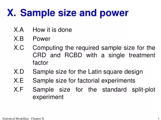
1. X. Sample size and power X.A How it is done X.B Power X.C Computing the required sample size for the CRD and RCBD with a single treatment factor X.D Sample size for the Latin square design X.E Sample size for factorial experiments X.F Sample size for the standard split-plot experiment Statistical Modelling Chapter X

2. X.A How it is done Example X.1 Penicillin yield • For experiments, sample size is abut finding the number of replicates, r. • In example IV.1 the effects of four treatments (A, B, C and D) on the yield of penicillin were investigated. • It was concluded that the following treatment means were not significant: • However, perhaps there are differences between the penicillin treatments • just that 5 replicates was not enough, given the size of the true differences between the treatment means. • How many replicates should we take? Statistical Modelling Chapter X

3. In order to compute the r you will have to specify: • the significance level, a; • the power (or probability of detecting a difference when there is actually a difference) desired, 1 -b; • the number of treatments to be investigated • the minimum size of the difference to be detected between a pair of treatment means, as measured by D; • the uncontrolled variation, , expected. Detemining no. replicates • Determine the number of pure replicates of a treatment, denoted r. • In working out values for these, often the results from a previous experiment, you or another researcher has run, will be useful. • With this information, use R function no.reps to compute, r. • It, and its associated functions power.exp and power.diff, are available in the dae library. Statistical Modelling Chapter X

4. Usage and arguments for no.reps no.reps(multiple=1, df.num=1, df.denom=expression((df.num+1)*(r-1)), delta=1, sigma=1, alpha=0.05, power =0.8, tol = 0.025, print=FALSE) • Note the values given to arguments are the defaults if the argument is not set in a call to the function. multiple: the multiplier, m, which when multiplied by the number of pure replicates of a treatment, r, gives the number of observations used in computing means for some, not necessarily proper, subset of the treatment factors; m is the replication arising from other treatment factors. However, for single treatment factor experiments the subset can only be the treatment factor and m = 1; df.num: the df of the numerator of the F for testing the term involving the treatment factor subset; df.denom: an expression for the df of the denominator of the F for testing the term involving the treatment factor subset • must involve r, the number of pure replicates, • can involve other arguments to no.reps such as multiple and df.num, • must be enclosed in an expression function so that it is not evaluated when no.reps is called but will be evaluated as different values of r are tried during execution of no.reps; delta: the true difference between a pair of means for some, not necessarily proper, subset of the treatment factors; sigma: population standard deviation; alpha: the significance level to be used; power: the minimum power to be achieved; tol: the maximum difference tolerated between the power required and the power computed in determining the number of replicates; print: TRUE or FALSE to have or not have a table of power calculation details printed out. Statistical Modelling Chapter X

5. Example X.1 Penicillin yield (continued) • We now determine the number of replicates required to achieve a power of 0.80 in detecting D= 5 with a= 0.05. • In the ANOVA for this experiment, the Residual MSq was 18.83 so we will take • Output from no.reps for the present example is as follows: > no.reps(multiple=1, df.num=3, + df.denom=expression(df.num*(r-1)), delta=5, + sigma=sqrt(20), power=0.8) • $nreps • [1] 19 • $power • [1] 0.8055926 • Required number of replicates is 19 with a power of 0.8056. Statistical Modelling Chapter X

6. X.B Power a) Type I and II errors • It is important to keep in mind that your conclusion about the null hypothesis is not 100% certain to be correct. • The possible outcomes — the conclusion (or verdict) reached as a result of a hypothesis test — are: • Thus there are two types of errors that can be made in performing a hypothesis test. Statistical Modelling Chapter X

7. Two types of errors • Definition X.1: A type I error is made when the null hypothesis is true and it is rejected. • The probability of a type I error is designated a and is: • Definition X.2: A type II error is made when the null hypothesis is false and it is not rejected. • The probability of a type II error is designated b and is: • In a hypothesis test we set the probability of a type I error at a, called the significance level. • So set the level of risk prepared to take in making a type I error. • But what about the probability of a Type II error, b? • Rather than b, often consider 1-b, called the power of the test. Statistical Modelling Chapter X

8. b) Power of a hypothesis test about expectation model terms • Definition X.3: The power of a hypothesis test is the probability of rejecting the null hypothesis when it is false is: • Now to compute this probability means that we need to know the condition under which the null hypothesis is rejected. Statistical Modelling Chapter X

9. Rejecting the null hypothesis • In general the null hypothesis is rejected when the computed value of the probability of the F statistics from the analysis of variance is less than a. • Will occur whenever observed F > a% value from the Snedecor’s F distribution. • In this case any observed value of the test statistic greater than 3.49 would result in a p-value of less than 0.05 and so be rejected at the 5% level. Statistical Modelling Chapter X

10. How false is the null hypothesis? • Know H0 is false. • That is, there are differences between the population treatment means. But, how big a difference? • For the single, treatment-factor experiments a measure of the size of the differences, relative to the magnitude of the uncontrolled variation, is given by • provided the number of replicates for all treatments is r. • However, to use this formula requires that we know the values of the ts which is unlikely as estimating these is the purpose of the experiment. Statistical Modelling Chapter X

11. Overcoming unknown ts • A way to overcome this is to specify D, the difference such that if any two population means differ by this amount, H0 should be rejected. • Then it can be shown that a general formula for the minimum value of l is • where • r is the number of pure replicates of each treatment • m is the multiplier of r that gives no. of observations (rm) used in computing one of the means. • For experiments involving a single treatment factor m= 1. • For a single, treatment-factor RCBD r=b. • For a single, treatment-factor LS r=t. Statistical Modelling Chapter X

12. F distribution when H0 is false • We can now be more specific about computing the power: P{H0 rejected | H0 false} • need the probability of getting a value of F greater than that of the a% value from Snedecor’s F distribution when there is a difference between the treatments of the order specified by D (or l). • Clearly, Snedecor’s distribution cannot be used to compute this probability as it is the distribution that applies when the null hypothesis is true and D= 0. • We need a distribution of F for when the null hypothesis is false. • This is provided by the noncentral F distribution • a modification of the (central) Snedecor's F distribution to incorporate a noncentrality parameter l. Statistical Modelling Chapter X

13. Shape of the noncentral F distribution • Depends on n1, n2 and l — for the central F distribution l= 0. • Distribution for: • l = 0 is distribution of F3,12 when H0 true • l= 4 is distribution of F3,12 when H0 is not true • l= 10 is distribution of F3,12 when H0 is even less true Statistical Modelling Chapter X

14. where is the F value from the central F distribution such that Computing the power • Specifically, to compute the power of an analysis of variance test for a fixed factor: • The R function pf computes probabilities for the noncentral F distribution • its arguments are q (= F), df1, df2 and ncp (= l). • Also, power.exp for computing power in an experiment — available in dae library. Statistical Modelling Chapter X

15. Usage and arguments for power.exp • power.exp(rm=5, df.num=1, df.denom=10, delta=1, sigma=1, alpha=0.05, print=FALSE) rm: the number of observations used in computing a mean. df.num: the degrees of freedom of the numerator of the F for testing the term involving the means; df.denom: the degrees of freedom of the denominator of the F for testing the term involving the means; delta: the true difference between a pair of means; sigma: population standard deviation; alpha: the significance level to be used print: TRUE or FALSE to have or not have a table of power calculation details printed out. Statistical Modelling Chapter X

16. Example X.1 Penicillin yield (continued) • Suppose expected that the minimum difference between a pair of treatment means for this experiment is 5 and that a = 0.05. • We continue to take • Also r= 5 and m= 1. Statistical Modelling Chapter X

17. need to set rm outside expression alpha not set in call — so default value of 0.05 used. 3 * (rm - 1) and sqrt(20) will be evaluated prior to call. l = 3.125 Example X.1 Penicillin yield (continued) • Output from power.exp call to compute power. > rm <- 5 > power.exp(rm=rm, df.num=3, df.denom=3*(rm-1), delta=5, + sigma=sqrt(20), print=TRUE) rm df.num df.denom alpha delta sigma lambda powr • 5 3 12 0.05 5 4.472136 3.125 0.2159032 [1] 0.2159032 • Power for detecting a minimum difference of 5 in a pair of treatment means when sU= 4.47 is 0.2159. Statistical Modelling Chapter X

18. Example X.1 Penicillin yield (continued) • No difference between treatments • probability of rejecting H0 determined from central F to be 0.05. • Treatment difference corresponding to l= 3.125 • probability of rejecting H0 determined from noncentral F to be 0.2159. Statistical Modelling Chapter X

19. Leads us to conclude that, for a fixed number of treatments, the noncentrality parameter will increase if • increase the number of replicates, r; • increase the size of the differences between the treatments, as measured by D; • decrease the uncontrolled variation, . How can we improve power? • The power of the hypothesis test being 0.22 is not good because not a high chance of correctly rejecting H0. • Examine formula for noncentrality parameter • So we can get better power by changing these. • How can these be improved? • Most often have to increase r. Statistical Modelling Chapter X

20. Given the discussion on the power of a hypothesis test, as already noted, in order to compute the r you will have to specify: • the significance level, a; • the power desired, 1 -b; • the number of treatments to be investigated • the minimum size of the difference to be detected between a pair of treatment means, as measured by D; • the uncontrolled variation, , expected. X.C Computing the required sample size for the CRD and RCBD with a single treatment factor • As before, determining sample size amounts to determining number of pure replicates of a treatment, denoted r. • Achieved by computing the power for different rs until smallest r that has at least the required power is identified. • In working out values for these, often the results from a previous experiment, you or another researcher has run, will be useful. Statistical Modelling Chapter X

21. Using R to compute required r • Can be achieved by computing the power for different r s using the function power.exp • If the computed the power for a particular r is: • too high, decrease r, or • too low, increase r, continuing in both cases until you have identified the smallest r that has at least the required power. Statistical Modelling Chapter X

22. Example X.1 Penicillin yield (continued) • We now determine the number of replicates required to achieve a power of 0.80 in detecting D= 5 with a= 0.05. • We continue to take • 5 replicates achieved a power of only 0.22 and is clearly much smaller than required. Statistical Modelling Chapter X

23. Example X.1 Penicillin yield (continued) • Take r = 15 as our first guess and find that this would provide a power of 0.6860. > rm <- 15 > power.exp(rm=rm, df.num=3, df.denom=3*(rm-1), + delta=5, sigma=sqrt(20)) [1] 0.6860223 • Next increase r to 20 and this indicates a power of 0.8289 will be achieved. > rm <- 20 > power.exp(rm=rm, df.num=3, df.denom=3*(rm-1), + delta=5, sigma=sqrt(20)) [1] 0.828869 • As this is in excess of the required power, r is reduced to 19 and the power reduces to 0.8056. • As this is still in excess of the required power, r is reduced to 18 and the power reduces to 0.7798. • Clearly, 19 replicates is required to achieve a power of at least 0.80 — fewer will have less power. • More convenient method is provided by function no.reps. Statistical Modelling Chapter X

24. Example X.1 Penicillin yield (continued) • Output from no.reps for the present example is as follows: > no.reps(multiple=1, df.num=3, df.denom=expression(df.num*(r-1)), delta=5, + sigma=sqrt(20), power=0.8, print=TRUE) rm df.num df.denom alpha delta sigma lambda powr 1 20.33437 3 58.0031 0.05 5 4.472136 12.70898 0.836116 rm df.num df.denom alpha delta sigma lambda powr 1 31.66563 3 91.9969 0.05 5 4.472136 19.79102 0.9676862 rm df.num df.denom alpha delta sigma lambda powr 1 13.33126 3 36.99379 0.05 5 4.472136 8.33204 0.6226844 rm df.num df.denom alpha delta sigma lambda powr 1 22.64998 3 64.94994 0.05 5 4.472136 14.15624 0.8795446 rm df.num df.denom alpha delta sigma lambda powr 1 17.65942 3 49.97826 0.05 5 4.472136 11.03714 0.7704095 rm df.num df.denom alpha delta sigma lambda powr 1 18.62379 3 52.87137 0.05 5 4.472136 11.63987 0.7961913 rm df.num df.denom alpha delta sigma lambda powr 1 18.92537 3 53.77612 0.05 5 4.472136 11.82836 0.8037564 rm df.num df.denom alpha delta sigma lambda powr 1 18.77872 3 53.33616 0.05 5 4.472136 11.7367 0.8001066 rm df.num df.denom alpha delta sigma lambda powr 1 18.74539 3 53.23616 0.05 5 4.472136 11.71587 0.7992694 rm df.num df.denom alpha delta sigma lambda powr 1 18.81205 3 53.43616 0.05 5 4.472136 11.75753 0.800941 rm df.num df.denom alpha delta sigma lambda powr 1 18.77872 3 53.33616 0.05 5 4.472136 11.7367 0.8001066 $nreps [1] 19 $power [1] 0.8055926 • Confirms required number of replicates is 19 with a power of 0.8056. Statistical Modelling Chapter X

25. X.D Sample size for the Latin square design • Formulae for computing the power and sample size for an RCBD also apply to the Latin square except that the number of replicates is t. • However, number of rows, columns and treatments must be equal. • So you cannot increase the treatment replication without changing the number of treatments. • Consequently, main interest will be determine if the proposed design will have the desired power. • Use the function power.exp. Statistical Modelling Chapter X

26. X.E Sample size for factorial experiments • Sample size for a two-way factorial experiment can be computed using the R function no.reps. • Similar to the single, treatment-factor experiments described in the previous sections. • First step is to determine which effects you wish to specify to be determined with a nominated power: A main, B main and/or interaction effects. • Then determine the power for each set of effects. Statistical Modelling Chapter X

27. Note that for • A and B, D is the difference between a pair of A or B means. • A#B interaction, D is the difference between the simple effect for one of the factors and the corresponding main effect for that factor. • For example, • represents the difference between an A simple effect and the A main effect. Cells that vary for the different types of effects Statistical Modelling Chapter X

28. Example VII.4 Animal survival experiment • Poison and Treatment did not interact in their effect on the death rate. • However, consider the following combined table of means. • Main effect for Treats 2 vs 3: 2.947 – 1.862 = 1.085. • If no interaction, would expect differences between Treats 2 and 3 for each Poison to be about 1.085. • They are not exactly all equal to this value. • But, how different from 1.085 would be an important difference? This is what D is. Statistical Modelling Chapter X

29. DF denominator depends on design employed Statistical Modelling Chapter X

30. Example X.2 Fertilizing oranges • Suppose that for the experiment to investigate 3 levels of N and 2 levels of P, outlined in example VII.1, you wish to determine the number of blocks to use in an RCBD. • Like to be able to detect with 80% power, a difference between a simple effect and a main effect of 10. • You believe that the standard deviation will be about 7.5 and you will use a significance level of 5%. • How many replicates are required to achieve the desired power? • So we require the number of blocks in an RCBD to detect an interaction effect. • The R output for obtaining this is as follows: > no.reps(multiple=1, df.num=2, df.denom=expression(5*(r-1)), + delta=10, sigma=7.5, power=0.80) $nreps [1] 12 $power [1] 0.819291 • So 12 blocks needed to detect, with 80% power, a difference of 10 between a simple effect and a main effect. Statistical Modelling Chapter X

31. Determining the sample size for the standard split-plot experiment is complicated as involve 2 sources of uncontrolled variation: • main-plot variation • subplot variation X.F Sample size for the standard split-plot experiment • Require guesstimates of these two variances. • Then sample sizes computed as described for ordinary factorial experiments in section X.E • except that the values of the variance (s2) are varied as follows. Statistical Modelling Chapter X

32. X.G Exercises • Ex. 10-1 asks you to compute the sample size for an RCBD. • Ex. 10-2 asks you to compute the power for an RCBD. • Ex. 10-3 asks you to determine if a Latin square has adequate power. • Ex. 10-4 asks you to determine if a repeated Latin square has adequate power. • Ex. 10-5 asks you to compute the number of replicates for a factorial experiment laid out as a CRD. Statistical Modelling Chapter X