Martin Ott
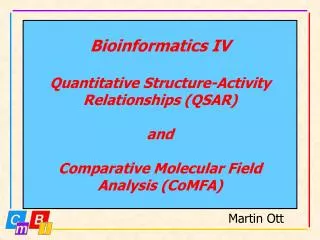
Bioinformatics IV Quantitative Structure-Activity Relationships (QSAR) and Comparative Molecular Field Analysis (CoMFA). Martin Ott. Outline. Introduction Structures and activities Regression techniques: PCA, PLS Analysis techniques: Free-Wilson, Hansch

Martin Ott
E N D
Presentation Transcript
Bioinformatics IVQuantitative Structure-Activity Relationships (QSAR)andComparative Molecular Field Analysis (CoMFA) Martin Ott
Outline • Introduction • Structures and activities • Regression techniques: PCA, PLS • Analysis techniques: Free-Wilson, Hansch • Comparative Molecular Field Analysis
QSAR: The Setting Quantitative structure-activity relationships are used when there is little or no receptor information, butthere are measured activities of (many) compounds They are also useful to supplement docking studies which take much more CPU time
QSAR: Which Relationship? Quantitative structure-activity relationships correlate chemical/biological activitieswith structural features or atomic, group ormolecular properties within a range of structurally similar compounds
Free Energy of Binding andEquilibrium Constants The free energy of binding is related to the reaction constants of ligand-receptor complex formation: DGbinding = –2.303 RT log K = –2.303 RT log (kon / koff) Equilibrium constant K Rate constants kon (association) and koff (dissociation)
Concentration as Activity Measure • A critical molar concentration Cthat produces the biological effectis related to the equilibrium constant K • Usually log (1/C) is used (c.f. pH) • For meaningful QSARs, activities needto be spread out over at least 3 log units
Molecules Are Not Numbers! Where are the numbers? Numerical descriptors
An Example: Capsaicin Analogs MR = molar refractivity (polarizability) parameter; p = hydrophobicity parameter; s= electronic sigma constant (para position); Es = Taft size parameter
An Example: Capsaicin Analogs log(1/EC50) = -0.89 + 0.019 * MR + 0.23 * p + -0.31 * s + -0.14 * Es
Basic Assumption in QSAR The structural properties of a compound contributein a linearly additive way to its biological activity provided there are no non-linear dependencies of transport or binding on some properties
Molecular Descriptors • Simple counts of features, e.g. of atoms, rings,H-bond donors, molecular weight • Physicochemical properties, e.g. polarisability,hydrophobicity (logP), water-solubility • Group properties, e.g. Hammett and Taft constants, volume • 2D Fingerprints based on fragments • 3D Screens based on fragments
Principal Component Analysis (PCA) • Many (>3) variables to describe objects= high dimensionality of descriptor data • PCA is used to reduce dimensionality • PCA extracts the most important factors (principal components or PCs) from the data • Useful when correlations exist between descriptors • The result is a new, small set of variables (PCs) which explain most of the data variation
Different Views on PCA • Statistically, PCA is a multivariate analysis technique closely related to eigenvector analysis • In matrix terms, PCA is a decomposition of matrix Xinto two smaller matrices plus a set of residuals: X = TPT + R • Geometrically, PCA is a projection technique in which X is projected onto a subspace of reduced dimensions
Partial Least Squares (PLS) (compound 1) (compound 2) (compound 3) … (compound n) y1 = a0 + a1x11 + a2x12 + a3x13 + … + e1 y2 = a0 + a1x21 + a2x22 + a3x23 + … + e2 y3 = a0 + a1x31 + a2x32 + a3x33 + … + e3 … yn = a0 + a1xn1 + a2xn2 + a3xn3 + … + en Y = XA + E X = independent variables Y = dependent variables
PLS – Cross-validation • Squared correlation coefficient R2 • Value between 0 and 1 (> 0.9) • Indicating explanative power of regression equation With cross-validation: • Squared correlation coefficient Q2 • Value between 0 and 1 (> 0.5) • Indicating predictive power of regression equation
Free-Wilson Analysis log (1/C) = S aixi + m xi: presence of group i (0 or 1) ai: activity group contribution of group i m: activity value of unsubstituted compound
Free-Wilson Analysis • Computationally straightforward • Predictions only for substituents already included • Requires large number of compounds
Hansch Analysis Drug transport and binding affinity depend nonlinearly on lipophilicity: log (1/C) = a (log P)2 + b log P + c Ss + k P: n-octanol/water partition coefficient s: Hammett electronic parameter a,b,c: regression coefficients k: constant term
Hansch Analysis • Fewer regression coefficients needed for correlation • Interpretation in physicochemical terms • Predictions for other substituents possible
Pharmacophore • Set of structural features in a drug molecule recognized by a receptor • Sample features: • H-bond donor • charge • hydrophobic center • Distances, 3D relationship
Pharmacophore Selection Pharmacophore Dopamine L = lipophilic site; A = H-bond acceptor; D = H-bond donor; PD = protonated H-bond donor
Pharmacophore Selection Pharmacophore Dopamine L = lipophilic site; A = H-bond acceptor; D = H-bond donor; PD = protonated H-bond donor
Comparative Molecular Field Analysis (CoMFA) • Set of chemically related compounds • Common pharmacophore or substructure required • 3D structures needed (e.g., Corina-generated) • Flexible molecules are “folded” intopharmacophore constraints and aligned
CoMFA Grid and Field Probe (Only one molecule shown for clarity)
CoMFA Model Derivation • Molecules are positioned in a regular gridaccording to alignment • Probes are used to determine the molecular field: Electrostatic field (probe is charged atom) Van der Waals field (probe is neutral carbon) Ec = S qiqj / Drij Evdw = S (Airij-12 - Birij-6)
CoMFA Pros and Cons • Suitable to describe receptor-ligand interactions • 3D visualization of important features • Good correlation within related set • Predictive power within scanned space • Alignment is often difficult • Training required