Download
1 / 34
340 likes | 701 Vues
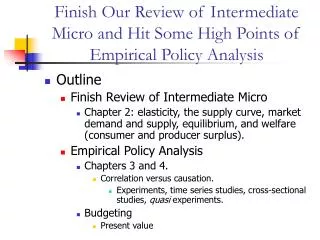
Finish Our Review of Intermediate Micro and Hit Some High Points of Empirical Policy Analysis Outline Finish Review of Intermediate Micro Chapter 2: elasticity, the supply curve, market demand and supply, equilibrium, and welfare (consumer and producer surplus). Empirical Policy Analysis

E N D
Finish Our Review of Intermediate Micro and Hit Some High Points of Empirical Policy Analysis • Outline • Finish Review of Intermediate Micro • Chapter 2: elasticity, the supply curve, market demand and supply, equilibrium, and welfare (consumer and producer surplus). • Empirical Policy Analysis • Chapters 3 and 4. • Correlation versus causation. • Experiments, time series studies, cross-sectional studies, quasi experiments. • Budgeting • Present value
EQUILIBRIUM AND SOCIAL WELFARE: Elasticity of demand • A key feature of demand analysis is the elasticity of demand. It is defined as: • That is, the percent change in quantity demanded divided by the percent change in price. • Demand elasticities are: • Typically negative numbers. • Not constant along the demand curve (for a linear demand curve). • It is easy to define other elasticities (income, cross-price, etc.).
EQUILIBRIUM AND SOCIAL WELFARE: Supply curves • We do a similar drill on the supply side of the market. Firms have a production technology (we might write it as) • We can construct isoquants, which represent the ability to trade off inputs, fixing the level of output. • The isocost function represents the combinations of various inputs, where total costs are fixed. • Firms maximize profit (minimize cost) when the marginal rate of technical substitution equals the input price ratio. • Also MR=MC at the profit-maximizing level of output.
EQUILIBRIUM AND SOCIAL WELFARE Equilibrium • In equilibrium, we horizontally sum individual demand curves to get aggregate demand. • We also horizontally sum individual supply curves to get aggregate supply. • A firm’s supply curve is the MC curve above minimum average variable cost. • Competitive equilibrium represents the point at which both consumers and suppliers are satisfied with the price/quantity combination. • Figure 21 illustrates this.
Equilibrium with Supply and Demand Figure 21 PM Supply curve of movies Intersection of supply and demand is equilibrium. PM,3 PM,2 PM,1 Demand curve for movies QM,3 QM,2 QM,1 QM
EQUILIBRIUM AND SOCIAL WELFARE: Social efficiency • Measuring social efficiency is computing the potential size of the economic pie. It represents the net gain from trade to consumers and producers. • Consumer surplus is the benefit that consumers derive from a good, beyond what they paid for it. • Each point on the demand curve represents a “willingness-to-pay” for that quantity. • Figure 22 illustrates this.
Deriving Consumer Surplus Figure 22 PM The consumer’s “surplus” from the first unit is this trapezoid. Yet the actual price paid is much lower. The willingness-to-pay for the first unit is very high. Supply curve of movies There is still surplus, because the price is lower. The willingness to pay for the second unit is a bit lower. The consumer’s “surplus” from the next unit is this trapezoid. The consumer surplus at Q* is the area between the demand curve and market price. The total consumer surplus is this triangle. P* Demand curve for movies 0 1 2 Q* QM
EQUILIBRIUM AND SOCIAL WELFARE: Social efficiency • Producer surplus is the benefit derived by producers from the sale of a unit above and beyond their cost of producing it. • Each point on the supply curve represents the marginal cost of producing it. • Figure 24 illustrates this.
Producer Surplus Figure 24 PM Supply curve of movies The producers surplus at Q* is the area between the demand curve and market price. The total producer’s surplus is this triangle. P* There is producer surplus, because the price is higher. The marginal cost for the second unit is a bit higher. The producer’s “surplus” from the next unit is this trapezoid. The producer’s “surplus” from the first unit is this trapezoid. The marginal cost for the first unit is very low. Yet the actual price received is much higher. Demand curve for movies 0 1 2 Q* QM
EQUILIBRIUM AND SOCIAL WELFARE: Social efficiency • The total social surplus, also known as “social efficiency,” is the sum of the consumer’s and producer’s surplus. • Figure 25 illustrates this.
Social Surplus Figure 25 PM Providing the first unit gives a great deal of surplus to “society.” The surplus from the next unit is the difference between the demand and supply curves. Supply curve of movies Social efficiency is maximized at Q*, and is the sum of the consumer and producer surplus. The area between the supply and demand curves from zero to Q* represents the surplus. P* This area represents the social surplus from producing the first unit. Demand curve for movies 0 1 Q* QM
EQUILIBRIUM AND SOCIAL WELFARE: Competitive equilibrium maximizes social efficiency • The First Fundamental Theorem of Welfare Economics states that the competitive equilibrium, where supply equals demand, maximizes social efficiency. • Any quantity other than Q*reduces social efficiency, or the size of the “economic pie.” • Consider restricting the price of the good to P´<P*. • Figure 26 illustrates this.
Deadweight Loss from a Price Floor Figure 26 PM Supply curve of movies This triangle represents lost surplus to society, known as “deadweight loss.” The social surplus from Q’ is this area, consisting of a larger consumer and smaller producer surplus. With such a price restriction, the quantity falls to Q´, and there is excess demand. P* P´ Demand curve for movies Q´ Q* QM
EQUILIBRIUM AND SOCIAL WELFARE: The role of equity • Societies usually care not only about how much surplus there is, but also about how it is distributed among the population. • Social welfare is determined by both criteria. • The Second Fundamental Theorem of Welfare Economics states that society can attain any efficient outcome by a suitable redistribution of resources and free trade. • In reality, society often faces an equity-efficiency tradeoff.
EQUILIBRIUM AND SOCIAL WELFARE The role of equity • Society’s tradeoffs of equity and efficiency are models with a Social Welfare Function. • This maps individual utilities into an overall social utility function.
EQUILIBRIUM AND SOCIAL WELFARE The role of equity • The utilitarian social welfare function is: • The utilities of all individuals are given equal weight. • Implies that government should transfer from person 1 to person 2 as long as person 2’s gain is bigger than person 1’s loss in utility.
EQUILIBRIUM AND SOCIAL WELFARE The role of equity • Utilitarian SWF is maximized when the marginal utilities of everyone are equal: • Thus, society should redistribute from rich to poor if the marginal utility of the next dollar is higher to the poor person than to the rich person.
EQUILIBRIUM AND SOCIAL WELFAREThe role of equity • The Rawlsian social welfare function is: • Societal welfare is maximized by maximizing the well-being of the worst-off person in society. • Generally suggests more redistribution than the utilitarian SWF.
Chapter 3: Empirical Approaches to Policy Analysis • Empirical public finance is the use of data and statistical methodologies to measure the impact of government policy on individuals and markets. • Key issue in empirical public finance is separating causation from correlation. • Correlated means that two economic variables move together. • Casual means that one of the variables is causing the movement in the other.
THE IMPORTANT DISTINCTION BETWEEN CORRELATION AND CAUSATION • One interesting, tragic example given in the book describes some Russian peasants. • There was a cholera epidemic. Government sent doctors to the worst-affected areas to help. • Peasants observed that in areas with lots of doctors, there was lots of cholera. • Peasants concluded doctors were making things worse. • Based on this insight, they murdered the doctors.
The Problem • In the Russian peasant example, the possibilities might be: • Doctors cause peasants to die from cholera through incompetent treatment. • Higher incidence of illness caused more physicians to be present. • Peasants thought the first possibility was correct.
MEASURING CAUSATION WITH DATA WE’D LIKE TO HAVE: RANDOMIZED TRIALS • Randomized trials are one often effective way of assessing causality. • Trials typically proceed by taking a group of volunteers and randomly assigning them to either a “treatment” group that gets the intervention, or a “control” group that is denied the intervention. • With random assignment, the assignment of the intervention is not determined by anything about the subjects. • As a result, with large enough sample sizes, the treatment group is identical to the control group in every facet but one: the treatment group gets the intervention.
The Problem of Bias • Bias represents differences between treatment and control groups that is correlated with the treatment, but not due to the treatment. • An example of bias: in 1988 the SAT scores of Harvard applicants who took test preparation courses were lower than those of students who did not. This would bias straightforward effort to study the effects of SAT classes on test scores. • By definition, such differences do not exist in a randomized trial, since the groups, if large enough, are not different in any consistent fashion.
Why We Need to Go Beyond Randomized Trials • Randomized trials present some problems: • They can be expensive. • They can take a long time to complete. • They may raise ethical issues (especially in the context of medical treatments). • The inferences from them may not generalize to the population as a whole. • Subjects may drop out of the experiment for non-random reasons, a problem known as attrition.
Time Series Analysis • Time series analysis documents the correlation between the variables of interest over time. • It is difficult to identify causal effects when there are slow moving trends and other factors are changing. • Sharp changes in a policy variable over time, may create opportunities for valid inference.
Cross-Sectional Regression Analysis • Cross-sectional regression analysis is a statistical method for assessing the relationship between two variables while holding other factors constant. • “Cross-sectional” means comparing many individuals at one point in time. • An example: • Where the control variables account for race, education, age, and location
Quasi-Experiments • Economists typically cannot set up randomized trials for many public policy discussions. Yet, the time-series and cross-sectional approaches are often unsatisfactory. • Quasi-experiments are changes in the economic environment that create roughly identical treatment and control groups for studying the effect of that environmental change. • This allows researchers to take advantage of randomization created by external forces.
An Example of a Quasi-Experiment • New Jersey raises their state minimum wage. Pennsylvania does not. • We are interested in the effect of the minimum wage on employment. • We could look at the employment of low-skilled workers in NJ before and after the minimum wage increase. • But other things in the economy might be occurring. • So, we can see how employment changed in PN over the same interval. • The difference in employment in NJ, before and after, compared to the difference in employment in PN, before and after, may reveal the causal effect of minimum wages changes, if NJ and PN are identical (similar?) in other respects.
Structural Modeling • Both randomized trials and quasi-experiments suffer from two drawbacks: • First, they only provide an estimate of the causal impact of a particular treatment. It is difficult to extrapolate beyond the changes in policy. • Second, the approaches often do not tell us why the outcomes change. For example, the approaches do not separate out income and substitution effects in the TANF example used in the book. • Structural estimation attempt to estimate the underlying parameters of the utility function.
A Couple Items About Federal Budgets • Government debt is the amount that a government owes to others who have loaned it money. • It is a stock variable; the debt is an amount owed at any point in time. • Government deficit is the amount by which spending exceeds revenues in a given year. • It is a flow variable; the deficit flow is added to the previous year’s debt stock to produce a new stock of debt owed.
Real vs. Nominal • The debt and deficit are often expressed in nominal values–that is, in today’s dollars. • Inflation changes the real value of the debt or deficit, however, because prices change. • The consumer price index (CPI) measures the cost of purchasing a typical bundle of goods. It increased 91% between 1982 and 2003. • Inflation reduces the burden of the debt, as long as that debt is a nominal obligation to borrowers. • Rising prices leads to what is known as the “inflation tax” on the holders of the debt–the payments are worth less because of rising prices. • In 2003, the national debt was $3.91 trillion and inflation was 1.9%. The inflation tax was therefore $74 billion, which would reduce the conventionally measured deficit from $375 billion to $301 billion.
Background: Present Discounted Value • To understand budgeting, you must understand the concept of present discounted value (PDV). • Receiving a dollar in the future is worth less than receiving it today, because you have foregone the opportunity to earn interest. • PDV takes future payments and expresses them in today’s dollars. • It does so by discounting payments in some future period by the interest rate.
Background: Present Discounted Value • A stream of payments would be discounted as: • Where B0 through Bt represent a stream of benefit obligations, r is the interest rate, and t is the number of periods. • For example, $1,000 received 7 years from now is only worth $513 with a 10% interest rate: • A constant payment received indefinitely has the PDV=P/r