Download

1 / 49
490 likes | 621 Vues
July 21, 2011. Study of g production in association with jets using the CMS detector. Michael Anderson. Outline. Standard Model of Particle Physics Events of photon + jets Large Hadron Collider Compact Muon Solenoid Detector Detector/Physics Simulation Measuring Jets and Photons

E N D
July 21, 2011 Study of g production in association with jets using the CMS detector Michael Anderson
Outline • Standard Model of Particle Physics • Events of photon + jets • Large Hadron Collider • Compact Muon Solenoid Detector • Detector/Physics Simulation • Measuring Jets and Photons • Conclusions
Standard Model • Quarks interact via Strong Force (g), leptons cannot • Quarks, e, m, t interact via Electromagentic Force (g) • Both quarks and leptons interact via Weak Force (W, Z) • Quarks are tightly bound can cannot be detected individually • Quarks combine to form composite particles • Examples: Quarks (Fermions) Force Carriers (Bosons) H Higgs Leptons (Fermions) proton neutron pion
Composite Particles proton • Probing composite particles (like protons) at high energy will find gluons and “sea” quarks • All quarks & gluons within hadrons referred to as “partons” • Parton Distribution Functions (PDFs): • defined as probability density for finding a particle with a certain momentum fraction, x, at a given momentum transfer • Must be determined experimentally • Needed as input to make theoretical predictions Simplified picture. In high-energy collisions, energy is available for finding “sea” quarks • x = p(parton)/p(hadron)
Photons and Jets • Prompt Photons: come directly from interaction • Energy & position can be measured accurately • Prompt, Isolated photons provide good probe of hard-scattering process (like pp collisions) • Jets: quarks and gluons fragment into collimated collection of hadrons • Must measure jets to determine momentum of original scattered parton • Non-prompt photons produced within jets (“jet”) Jet example
Motivation for g+jets • Motivation for study of photon+jet events includes: • Test/Validate theoretical predictions • Cross section calculations are challenging as the number of jets increases • Explore new kinematic regions in hadron-hadron collisions • They are background to pp->Higgs->gg • Also background for beyond standard model searches • Ability to constraining PDFs of the proton • Calibrate jet energy scales Prompt Photons Bremsstrahlung Photons • Prompt photons produced from quark-gluon scattering & quark-anti-quark annihilation • Primary prompt photon background comes from neutral meson decays
Goal • Goal: measurement of the rate of events in which a proton-proton collision produces a prompt photon and jets • Prefer to measure inclusive rate of jets (rate of events with ≥ n jets), and to not correct for acceptance of the detector
Large Hadron Collider • Circumference of 27 km • In 2010, collided protons with center-of-mass energy of 7 TeV • Protons are organized into bunches (next slide)
Proton Collisions at LHC Design Achieved 1380 bunch/beam 1.3*1011 3.5 TeV 1.3*1033 cm-2s-1 Luminosity L = particle flux/time Interaction rate Cross section, = “effective” area of interacting particles During 2010 run: Beam energy 3.5 TeV (7 TeV center of mass) Peak Luminosity, L = 2x1032 cm-2s-1 Recorded 36pb-1 of p-p collisions
Compact Muon Solenoid Solenoid (3.8T) Muon chambers Forward calorimeter Silicon Strip & Pixel Tracker Electromagnetic Calorimeter Hadronic CalorimeterBrass/Scintillator Weight: 12,500 metric tons Diameter: 15 m Length: 21.5 m
Compact Muon Solenoid ← Surface assembly hall CMS together underground ↓ Endcap Discs: Designed, assembled & installed by Wisconsin
Detector Geometry • Pseudorapidityh = -ln(tan(q/2) • Another common variable: • Radius: DR = ((Df)2 + (Dh)2)1/2(used for sizes of jets, for example) One quadrant slice of CMS parallel to proton beam pipe h=0.0 Slice of CMS perpendicular to beam pipe h=1.5 f=p/2 h=3.0 h=inf f=0
Particle Detection • Prompt Photons: • Deposit of of Energy in ECAL • Generally isolated from other energy deposits in Tracker, ECAL & HCAL • Found by clustering energy of ECAL crystals • Jets • Energy deposit in ECAL & HCAL • With tracks • Found by clustering tracks and energy deposits in the calorimeters • Detector returns quantities like transverse momentum, pT, and transverse energy, ET pp collisionpoint Slice of CMS perpendicular to proton beam pipe
Particle Flow Algorithm • Particles are found using Particle-Flow (PF) Algorithm • Collects information from all subdetectors • Tracker, ECAL, HCAL, and muon System • Information from each sub-detector is linked to find individual particles (e,g,m,charged & neutral hadrons) • Example: track is associated with ECAL deposit and so found an electron • All particles found are then available to be clustered with jet algorithms • Used “anti-kT” clustering algorithm
g+jet Characteristics • Prompt Photon is generally isolated deposit of energy in ECAL (red) • Jet is collimated collection of tracks (green), and deposit of energy in the ECAL (red) and HCAL (blue) • Events with 1 prompt photon and 1 jet have the photon and jet roughly opposite in f Slice of CMS perpendicular to beam pipe Jet Photon
Silicon Tracker • Measures pT & path of charged particles within |h| < 2.5 • Strip Tracker • 200 m2 coverage • 10m precision measurements • 11M electronic channels • Inner Pixel tracking system • 66M channels • Used for isolating prompt photons, and finding jets & measuring their pT
Electromagnetic Calorimeter =-ln(tan(/2) • Measures energy & position of electrons and photons within |h| < 3 • PbWO4 crystals, very dense (8.3 g/cm3) • 23 cm long (26 radiation lengths) • 61K in the barrel, 22 x 22 mm2 • 15K in the endcaps, 28 x 28 mm2 • Resolution:
Hadronic Calorimeter • Barrel and Endcap: brass & scintillator • Coverage to || < 3 • x =0.087x0.087 • Hadron Forward: steel & quartz fiber: coverage 3 < || < 5 • Also used for isolating photons and finding jets • Resolution on energy of a single particle:
Trigger • Level 1: Hardware trigger operating at bunch crossing rate (40MHz at design luminosity) • Brings event rate down to 50-100 kHz • Level 2: • Reconstruction done using High-Level Trigger (HLT) -- computer farm • Reduces rate from Level-1 value of up to 100 kHz to final value of ~300 to 400 Hz • Slower, but determines energies and track momenta to high precision
Level-1 Trigger • ~25 ns bunch crossings*2.2 interactions/crossing • Not all events can be stored/processed • L1 trigger electronics select 50-100 kHz of interesting events • e/g trigger: • 8 or 12 GeV threshold • ~100% efficient Calorimeter Trigger Muon Trigger RPC CSC DT HF HCAL ECAL Local CSC Trigger Local DT Trigger RegionalCalorimeterTrigger PatternComparator Trigger CSC TrackFinder DT TrackFinder GlobalCalorimeterTrigger 40 MHz pipeline, latency < 3.2 μs Global Muon Trigger e, J, ET, HT, ETmiss 4 m Global Trigger max. 100 kHz L1 Accept
Computing • CMS is dependent on computing for transmitting, storing, and processing data • Every collision event ~0.2MB, and we record ~300 events/s • Needs to be shared with ~2000 collaborators around the world • Uses “tiered” system to organize responsibilities among many computing facilities around the world • One Tier0: CERN • Several Tier1s: One per country, FNAL in US • Dozens of Tier2s: One is here at UW-Madison • I was involved with Tier2 responsibilities (production of montecarlo simulations for collaboration, support of end-user analysis…) Tier0: CERN Tier2: UW-Madison Tier1: Fermilab Many other computing facilities not shown
Data • Data entirely collected in 2010 • Total of 36 pb-1 of high quality data (all subdetectors working well) • Required events to pass a trigger requiring the presence of at least one high-energy photon • Trigger required a clustered deposit of energy that passes: • ET > minimum thresh (20 GeV in early runs, and raised as luminosity increased) • Ratio of Hadronic E to Electromagnetic E < 0.15 • Energy shape ratio (called ‘R9’) < 0.98 in barrel of CMS (to remove anomalous ‘spikes’ from ionization of APD’s in barrel of CMS)
Monte Carlo Predictions • Data is compared to predictions made by simulations of proton collisions • Simulations are made by software called Monte Carlo event generators • Two useful programs used in this analysis: • Pythia: simulates events of g+1 jet.Pythia can only simulate processes of 2->2. • Madgraph/Madevent: used to simulate g+n jets (n = 1 to 3).Madgraph does fixed order matrix element calculations of cross sections.Madgraph is interfaced to use Pythia for jet hadronization. • Both simulators used as input the same parton distribution functions • from the CTEQ collaboration Example diagram of a generated event
Analysis Steps • Select events with at least one photon passing selection, then count number of jets above a pT threshold • Select signal from data: • Determine fraction of signal & background by fitting a distribution in which signal & background have different shapes • Correct for selection efficiency • efficiency = (number of photons passing some selection) / (all true hard-scattering photons) • Unsmear the measured jet distributions to obtain a distribution that may be compared directly with theoretical predictions (called “unfolding”)
Analysis Flow Events • Final Plots: • σ(γ + ≥n jets) / σ(γ + ≥1 jets) • σ(γ + ≥n jets) / σ(γ + ≥(n-1) jets) • Where: • Ns=number of events with a prompt photon and n jets • U=Unsmearing (‘Unfolding’) correction • ε=Efficiency • Lint = integrated luminosity Event Selection Exclusive Njet distributions Find signal fraction Correct Njet dist. for efficiency Unfold Njet dist. Change Njet binning from exclusive to inclusive
Event Selection • Pass single photon trigger • Photon passing: • pT > 75 GeV • |h|<1.4442 or 1.566<|h|<2.5 • Measuring photons is problematic in boundary region • Energy Isolation [next slide] • Jet, if present: • pT > 30 GeV • |h| < 2.4 • Loose Jet Identification [next slide] • Standard selection to selection high-quality proton-proton collision events • Removes events where beam interacted with beam pipe • The presence of a vertex close to nominal interaction point (|z|<24cm) Endcap Barrel Endcap
Photon Selection • Photon Isolation quantities: • Sum of energy in cones aligned with a line from primary vertex to center of photon energy deposit in ECAL • Sums do not include small central region to avoid including photon energy itself • Radius of cone = 0.4 • Selection on isolation sums: • Track Iso < 2.0 GeV • EcalIso < 4.2 GeV • HcalIso < 2.2 GeV • Selection on photon energy itself: • Ratio of Hadronic E to Electromagnetic E < 0.05 To measure isolation of photon, energy is summed around the photon HCAL ECAL Tracker
Photon Selection • Isolation sums around photons • True photons generally have lower values while Jets have higher values Remove > 4.2 GeV Remove > 2.0 GeV Remove > 2.2 GeV
Jet Selection • Jets are collimated, clustered energy in the Tracker, ECAL, and HCAL within a maximum cone size of R = 0.5 • Jet selection is very loose, simply to remove noise or anomalous signals • Additional selection for jets: • Photon must not overlap with jet, DR(jet,leadg) > 0.5 • Jets not from the same pp collision were removed by requiring distance between jet vertex and event vertex < 0.2 cm • Charged HadronEnergyFraction > 0.0 • Charged Em Energy Fraction < 0.99 • Charged Multiplicity > 0 • Neutral Hadron Energy Fraction < 0.99 • Neutral EmEnergy Fraction < 0.99
Number of Events • Number of events left after each selection • Jets leave deposits of energy in ECAL which are background to true photons • Isolation requirements removes a significant amount of these
Lead photon; jet pT • pT distribution of lead photon and lead jet (if found) for both data and Madgraph MC • Used s from Madgraph to scale to data • Madgraph is leading-order and underestimates yield • Scaled by ~1.6 to better compare shapes • Will fit to a variable to determine amount of signal & background in data (shown in 2 slides) Prompt Photon Jet
Jet Multiplicity • Exclusive number of jets above pT threshold • Madgraph samples simulated up to g+3 jets • pT distribution for 2nd and 3rd leading jet is modeled by Madgraph reasonably well Jet Multiplicity 2nd Jet pT 3rd Jet pT
Signal Extraction • To measure number of signal event must measure fraction of signal in data • We use a shower-shape variable of the lead photon defined as sum over ECAL crystals in photon’s cluster: • Where: • Signal shower shape comes from MC, but background shape comes from data with a sideband selection Photon in Barrel Photon in Endcap
Fitting template variable • Fit σiηiη to determine fraction of signal in data • Used Extended Maximum-Likelihood fits • Fits are performed separately in Barrel and Endcap, and for each # of jets • Jet distributions then scaled by these fractions Photon in Barrel Photon in Endcap
Signal Fraction • Results of fits to σiηiη • Signal fraction was found to be generally higher in the barrel • Too few stats in the endcap for higher jet multiplicity • Used average of lower multiplicity bins
Efficiency Correction • Efficiency = number of prompt photons passing selection / all prompt photons • Photon isolation selection efficiency depend on number of jets • Ultimately had to use efficiency from MC for high energy photons, but checked efficiency from MC against data for low energy photons • Pure sample of photons is hard to get with amount of data available • However, electrons & photons leave similar energy deposits in ECAL, so it is reasonable to use sample of electrons to find efficiency • We can use events of ‘pp -> Z -> ee’ for very pure sample of electrons
Tag & Probe Fits • Found photon selection efficiency using events of pp -> Z -> ee • First, require the presence of electron passing tight selection • Next, require another electron which also came from the Z (the invariant mass of the electron pairs satisfy 60 < Minv(ee) < 120 GeV) • This method is called ‘Tag and Probe’ • Tag: Election passing tight selection & pT>20GeV • Probe: Electron with pT> 30 GeV • Also counted number of jets • Fits to invariant mass performed to determine amount of electrons before & after requiring probe electron to pass photon selecton
Eff of Loose Photon Iso Probe/g in Barrel • Efficiency of photon selection vs number of jets with pT>30GeV • Using fits to Z mass • For photons with pT > 30 GeV • Efficiency decreases by a few % as number of jets increases Probe/g in Endcap
Unsmearing Jet Multiplicity Madgraphg + jet Response Matrix • Due to detector resolution, number of jets found by detector may differ from number of generated jets • Must unsmear or ‘unfold’ to remove effects of measurement resolutions, systematic biases, and detection efficiency to determine “true” distribution • Shown here is a matrix from MC of number of generated jets vs number of measured jets • Called ‘response matrix’ • These are used to unsmear measured number of jets to obtain a distribution that can be compared to theory • Response matrices here from Pythia and Madgraph signal MC • rows are normalized to they sum to 1 for easy comparison
Unsmearing Jet Multiplicity • Performed unsmearing using Bayesian (“iterative”) method with 4 iterations • Unfolding has an effect of a few % at 1 or 2 jet multiplicities, up to 50% at highest multiplicities
Incl. Jet Multiplicity • Inclusive jet multiplicity, ratio of “≥njets” to “≥1jets” • Data is after all corrections and unfolding • Madgraph and Pythia comparison are with generated particles before any detector simulation • Data agrees well with madgraph up to ≥3jets • Pythia only simulates g+1 jet, and simulates showering
Incl. Jet Mult Ratio • Inclusive jet multiplicity ratio of “≥njets” to “≥(n-1)jets” • Data is after all corrections and unfolding • Madgraph and Pythia comparison are with generated particles before any detector simulation • Data agrees well with madgraph up to ≥3jets • Pythia only simulates g+1 jet, and simulates showering
Systematics • Largest Uncertainty is from uncertainty in jet energy • Affects the counting of jets above an pT threshold • Uncertainty of jet energy scale arises from: • Uncertainty in flavor composition between jets used to determine energy corrections and jets in γ+jets will add ~2% on uncertainty • Subtraction is performed remove 500 MeV to jets in events without pile–up, so we must add this to systematic uncertainty in jet energy • Uncertainty in energy corrections as function of jet η and pT • Uncertainty in efficiency of photon selection as function of number of jets • Uncertainty in signal fraction from different background template selection
Systematics Details • Systematics on ratio “(njet)/ ((n-1)jet)” • Jet Energy Scale (+/- 1s to jet energies) • Background Template (different selection for efficiency extraction) • Selection Efficiency (using PythiavsMadgraph) • Unfolding (using response matrix from PythiavsMadgraph)
Jet Multiplicity Results • Inclusive jet multiplicity agrees well with Madgraph in 2 &3 jet bins, data is higher than Madgraph in higher jet multiplicities • Systematics are higher for larger number of jets primarily due to jet energy uncertainty
From W/Z+Jets • Another CMS analysis found number of jets in events with W or Z • They also measured ratio of number of events of“x+ ≥n jets” to “x+ ≥(n-1) jets” where x=W or Z • Mine was the first to use photon + jets
Summary • Presented first measurement of jet rate in association with a high-pT photon • Results with 36pb-1 of data • Loose photon isolation selection • Jets with pT > 30 GeV, R=0.5, using anti-kT algorithm • Rates of jets in agreement with Madgraph simulations for ≥1 and ≥2 jets, but higher than predicted for ≥3 and ≥4 • This is expected because Madgraph sample used contains matrix elements for up to g+3jets • Data disagreement with Pythia is also expected because Pythia only simulates photon+1 jet, and uses showering to create more jets • Tuned Monte Carlo event generators can be used for new physics searches. Ex: • g+1 jet: background to H->gg • g+jets+missing ET: a signature for super-symmetry
MC Simulations • Events simulated with MadGraph • Fixed order matrix element calculations of cross sections • Generates multi-parton processes in hadronic collisions. • Hadronization simulation performed with Pythia 6 • Simulates development of underlying event • Generates jets from hadronization, also simulates parton showers, and initial and final state radiation • Detector simulated using GEANT4 • Toolkit for the simulation of the passage of particles through matter Hard scattering MadGraph Hadronization, showers, IFSR PYTHIA Detector simulation GEANT4 Reconstruction of event CMSSW