A cell constitutes the following

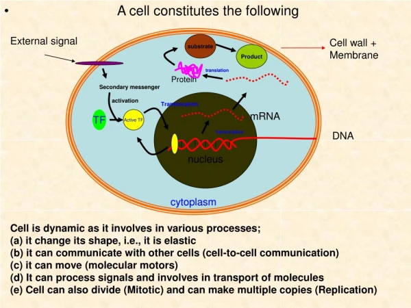
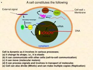
1. cytoplasm External signal substrate Cell wall + Membrane Product translation • A cell constitutes the following Protein Secondary messenger activation nucleus Translocation mRNA TF ActiveTF transcription DNA Cell is dynamic as it involves in various processes; (a) it change its shape, i.e., it is elastic (b) it can communicate with other cells (cell-to-cell communication) (c) it can move (molecular motors) (d) It can process signals and involves in transport of molecules (e) Cell can also divide (Mitotic) and can make multiple copies (Replication)

2. Genetic Info. • ‘GENETIC’ Information is also passed on from one generation to another through transcription and translational processes • ‘ENVIRONMENTAL’ Information flows in and out the cell through protein synthesis . Simplified version of earlier cell diagram. DNA mRNA Protein Regulation By proteins Physiology Transcription Translation Polypeptide Proteins (Inactive) Phosphorylation-dephosphorylation(P-D) acetylation Active (changes the conformation of protein)

3. Biological regulatory network (BRN) consists of sets of DNA’s, proteins and enzymes that involves in mutually regulating each other. • The regulation gives rise to (a) functioning of the cell at normal as well as in adverse conditions (b) set a stage for developmental by inducing phenotypic variations. • Regulation occurs at both transcription and translation. • Regulation involves multiple feedback loops • Feedback loops are classified as positive and negative. • Difficult to asess the complexity of feedback loops globally. • So intution alone is not sufficient to understand. Requires mathematical modelling. Various tools and methodologies are available for modelling.

4. Usefulness of Mathematical models in BRN’s • a) To account for experimental observations and to determine the validity of experimental conclusions. • (b) Clarification of hypothesis. • (c) Difficult to rely only on intuition. Mathematical equations provides a strong foundation for validating concepts and analyze complex data that involves multiple coupled variables. • (d) Models identify critical parameters for which certain phenomena can occur.

5. Different regulatory mechanisms can be explored through models from which only plausible mechanisms can be identified. This cannot be carried out through experiments, which are expensive and time consuming. • Models can help to identify different dynamically important regimes, which may be hard or inaccessible to experimentalists. • Models can suggest experimentalists to perform new experiments to explore unknown, but biologically important and interesting regimes. Conversely, it can also validate the suitability of the models. • Mathematical structure of the model helps to identify the similar regulatory processes that run through various biosystems

6. How to model BRN’s ? • Differential equations Ordinary (ODE) Partial (PDE) stochastic (SDE) Functional (FDE) Further can be classified as Linear and non-linear differential equations. To model GRN‘s the universal law of chemical mass action kinetics is used widely. To use mass action kinetics, static biological circuit diagramsshould be Constructed. To construct biological circuits, interaction among various proteins and types of interactions are necessary. This is transfomed in to mathematical equations.

7. In many systems, both positive and negative feedback loops together play an • Important role. • Take different types of positive and negative feedback loops and analyze for different dynamical phenomena. • Visualization is important for to understand biological systems. • Certain conclusion can be made by visualizing simple circuit diagrams. These • Circuit diagrams are the backbone and basis of large circuit diagrams. • After construction of biological circuit diagram, mathematical models are constructed. Models again can be visualized by two ways and are • Phase plane analysis (b) bifurcation diagrams. • We shall look at the first aspect now namely • Importance of feedback and inference from feedback circuit diagram and • the mathematical model based on feedback circuit diagram at a latter stage.

8. Classification of Feedback loops. Positive feedback loop brings about • Instability (explosive growth) • Amplification of a weak signal (c) Multistability (Multistationarity) and epigenetic modifications Negative feedback loop brings about • Homeostasis • Control the unexplosive growth • Induces oscillations (not in all cases) • Robust again perturbations.

9. Terminologies and classification Symbol Name Induction + DNA-Protein interaction - Repression gene g2 g1 m-RNA (Processed) Protein P1 P2 + Positive regulation Negative regulation Inhibition Protein-Protein interaction

10. g1 g2 p1 P2 g2 g1 P1 For present representation A B - - A B This circuit diagram is the abstraction of the whole network.

11. A B A B A B - - C + C What are the other circuits with feedback loops + Positive - negative Autregulatory feedback loop + Positive feedback loop A B + + - Negative feedback loop (daisy chain) + Feedback loops are determined by the parity of the negative signs

12. Two and three element feedback loops (non-homogenous or mixed feedback loops) - - + + A B A B + + Bistability Oscillations - + A B + + C Negative feedback loop Positive feedback loop Oscillations There is a common element ‘c’ that connects these feedback loops. It is called ‘Interlocked feedback loop’: Example is Circadian rhythms.

13. Some definitions Nonlinear dynamics: The rate of change of variables can be written as the linear function of the other related variables. Most nonlinear systems exhibit interesting dynamics like bistability and oscillations. Fixed point: It is the point where the rate of change of all variables are exactly Zero. Small perturbations of the fixed point will bring the system back to the same point and perturbations are quenched. It is then called stable. Multistability: Having more than one fixed point. Bistability: A system that has two stable fixed points.

14. Phase plane analysis. Its a graphical approach and can be only performed only for 2D systems. Its only a qualitative analysis. Its only for autonomous system. Where time does not occur explicitly in the differential equations. For example x y Right hand side of this equation, ‘t’ is not involved. The plot of x .vs. y gives the phase plane The trajectories in the phase plane is called the phase portrait. To find the critical points or steady state or Equilibrium points Trajectory

15. Linear Stability Analysis Eigen value Eigen vector Example of linear system This is the assumed solution coupled Linear Equations Characteristic Equation Matrix form of coupled Linear Equations Characteristic polynomial Very important Matrix!!!!! Eigen Values To determine Steady state Or Fixed point

16. Example: 1 Critical Point Called as STABLE NODE Equation Trajectories Starting from Different Initial conditions Matrix form Equilibrium Point Phase potraint Eigen values REAL,SAME SIGN AND UNEQUAL IC-1 Eigen vectors For different Eigen values IC-2 THE DYNAMICAL STATE IS STABLE NODE Time series

17. Example :2 Critical Point Called as SADDLE POINT Equation Matrix form Equilibrium Point Phase potrait Eigen values REAL, OPPOSITE SIGN AND UNEQUAL Eigen vectors For different Eigen values THE DYNAMICAL STATE IS SADDLE POINT Time series

18. Example :3 Critical Point Called as Stable Spiral Equation -0.5 1 -1 -0.5 A = Matrix form Equilibrium Point Phase potrait Eigen values REAL, and COMPLEX THE DYNAMICAL STATE IS STABLE SPIRAL/ FOCUS If the real part of eigen value is positive Then the critical point is unstable Spiral / Focus. Time series

20. Suppose if it is nonlinear equation, how to determine various dynamical states. It is Simple: Linearize nonlinear system around steady state. Linear stability analysis around the steady states using Taylor expansion. What is Taylors expansion ? Consider a function f(x,y) and expand around steady state (x*,y*).

21. This is the final form of the linearized • Nonlinear equation at the steadystate • Two things are to be determined • Jacobian • Eigen values of the characterestic • Equation.

22. Two steady states Example 4: Lotka-volterra Prey-predator model Jacobian Fixed or Equilibrium points for Is a saddle Eigenvalues for Is a Center/oscillatory Eigenvalues

23. Time series and phase portrait for α = 2, β =0.002, γ = 0.0018 and δ =2 In three dimension with time as the axis

24. A B A B - - C NATURE OF FEEDBACK LOOPS AND DYNAMICS • What dynamics is expected when • Self regulatory feedback loop • mutual induction / mutual repression • Three elements repressing each other in a daisy chain or • activationg each other in a daisy chain • Difficult to perform experiments unless certain predictions can be made • These predictions are • What conditions will bring bistability ? • (b) What conditions will bring about oscillations ? • Use mathematical models to findout and use the guidelines to • Build the regulatory circuit. • So (a) first find a naturally occuring simple circuit. • (b) Modify the circuit to build the circuit that exhibit desired dynamics. + A

25. Nomenclature that are to be known for understanding Gene regulation Ecoli • E.Coli, a prokaryotic system has • A single circular chromosome • (b) PLASMIDS, an extrachromosomanal DNA • (Usually this is manipulated to design new circuits) • Genes are referred in lower case italics, while proteins are referred in Uppercase. • For example,

26. Some terms you need to Know

27. (Cluster or group of genes)

28. How gene expression is monitored Gene expression is monitored through tagging the expressed gene with GREEN FLOURESCENT PROTEIN (GFP) Various variants are also available, but the principle is same. For example, Inducer P O When Gene expresses, then GFP also expresses with almost same quantitative amount. GENE GFP (Direction of expression) Flourescent Intensity Inducer

29. PARALLEL BETWEEN ENGINEERING TERMINOLOGIES Examples

30. CONSTRUCTION OF SYNTHETIC GENE CIRCUITS GUIDED BY MATHEMATICAL MODELS

31. Naturally ocurring system Two genes cI and cro Are under the control Of promoter PR and PRM. Cro and λ-rep binds to the Promoter and regulates Each other production. Cro λ High Low State Cro λ Lysis λ Cro Lytic Natural system Exhibits bistability Either can be in Lytic stage or Lysogenic state.

32. Classification of positive and negative feedback loops One element autoregulatory feedback loop + Positive - negative A B (Exhibits stability) (Exhibits bistability) Natural system Analogy: Water flowing on all directions from a tub due to holes. Control the flow to one direction by blocking all the holes except one. Tetracycline responsive transactivator Modified system High inducer concentration Low inducer concentration No regulation Feedback regulation regulated unregulated

33. Two element feedback loop (homogeneous) GENETIC TOGGLE SWITCH + ON A B [A] A B bistability Off + P + x + = + (Positive feedback loop) - x - = + (Positive feedback loop) Steady states (SS- I and II) can be seen in experiements, but unstable steady state (USS) cannot be seen in the experiments, but realized in mathematical model. ON ON [A] Off Off Stimulus SWITCH GRADED RESPONSE HYSTERESIS

34. Derivation of the box equation in Gardner paper. Circuit diagram R2 (R1) (P1) (P2) Kinetic equations Reducing to Dimensionless quantity Final box equation P M1 + P M1 R1 R1γ + p2 R1γp2 P = Promoter R = repressor Conservation equations Questions When bistability Occurs? What should be taken Care when plasmids Are constructed for Toggle switch Rate of synthesis

35. Interpretations Lumped parameters describes RNA-binding, transcript and polypeptide elongation, etc. Cooperativity from multimerization Of repressor protein and and DNA and Repressor binding Nullcline of above equations i.e., BISTABILITY MONO STABILITY Intersects at three points and isdue To cooperative effect, i.e., Two SS and one USS Bistability is possible only when the Rate of synthesis of two repressors are balanced. If not, only mono stability is obtained

36. Two parameter bifurcation diagram (Formation of Cusp) Large region CUSP bifurcation Rate of repressors if balanced properly, large region of bistability Is possible Slopes of the bifurcation lines are determined by the cooperativity Effect; High cooperativity effect, large bistable regime and vice versa Contributes to the robustness of the system.

37. Experimental observations of Synthetic toggle switch u v Natural What is observed in natural bacteriophage lambda circuit This is the constructed synthetic toggle switch by R-DNA technology taking into account of the theoretical considerations from model Toggle switch observed in experiments and variations is seen by monitoring Green flourescent protein (GFP). Synthetic Inducer LacI Clts GFP State IPTG high low high ON Heat Low high low OFF (Isopropyl B-D-thiogalactopyroniside)

38. First synthetic construct from the model and good prediction is made about the rate of synthesis and repressor stength for the occurrence of toggleswitch But predicted only average behavior of the cell and variations about the average cannot be predicted. For example, the time required for switching Toggle to high state for IPTG takes 3-6 hrs for different cells. Non-deterministic effects cannot be predicted. The switching time is very slow and is not useful for practical purpose. So different toggle switch was constructed which was temperature sensitive. Theswitching time is fast and rapid. Slow inductiontime And variability wwith IPTG Cell to cell variation with IPTG Fast induction time With temperature

39. Three element feedback loops (homogenous) - + A B A B - + - + C C negative feedback loop Positive feedback loop Oscillations [A] [A] (USS) SS-I (Off state) P P

40. - A B - - C Numerical and Experimental observation of Repressilator Leakiness For standard parameter Decrease in cooperativity Decrease in Repression i.e., > 0

41. Prediction from the model • Presence of strong promoters that binds the protein • (b) High cooperative binding of the repressors increases the range of • oscillatory regime and robustness • (c) The life time of the mRNA and proteins should be similar • for strong oscillations • Synthetic network that are to oscillate should be in accordance • to the above condition

42. Design of Experimental system Single cell isolated from colony flouresence Brigh field But there is a large variation in the cell. This is due to stochastic fluctuations of the molecules When simulated with stochastic model, this variation is accounted for.

43. Since this oscillator is noisy and unstable. ‘Hysteretic’ based oscillator Is proposed. Hypothetical network is constructed and the where the degradation of the Protein is controlled by a ‘slow’ subsytem. This gives ‘Relaxation oscillation’ Still there is no experimental evidence.