Detecting Dynamical Changes in Student Performance Using ARIMA: A Case Study in Education
20 likes | 139 Vues
This research aims to develop a methodology to analyze effects of interventions on student performance in small-enrollment courses. The study uses ARIMA analysis and cluster analysis to identify and measure changes in student responses. Data collection involves students rating their confidence in multiple-choice answers. The study identifies peaks and interferences in performance evolution, despite limitations due to practice effects. ARIMA models and Box-Jenkins procedure are employed for structural shift identification. The class-averaged ratings are viewed as a 'Dow Jones Index' for the class, which is modeled using ARIMA for analysis. Results from the analysis show shifts in performance sections, supporting visual identifications.

Detecting Dynamical Changes in Student Performance Using ARIMA: A Case Study in Education
E N D
Presentation Transcript
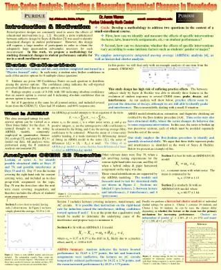
Time-Series Analysis: Detecting & Measuring Dynamical Changes in Knowledge Dr. Aaron Warren Purdue University North Central Dept. of Mathematics, Statistics, & Physics email: awarren@pnc.edu Introduction & Motivation • Goals: Develop a methodology to address two questions in the context of a small-enrollment course. • First, how can we identify and measure the effects of specific interventions (lectures, labs, homework assignments, etc.) on student performance? • Second, how can we determine whether the effects of specific interventions vary according to some intrinsic factors such as students’ gender or major? We employ autoregressive integrated moving average (ARIMA) analysis [4], as well as hierarchal cluster analysis. Pretest-posttest designs are commonly used to assess the effects of educational interventions [e.g., 1,2]. Recently, a more sophisticated between-subjects design by Sayre & Heckler [3] was used to identify dynamical changes in student performance. However, this design still requires a large number of participants in order to obtain the adequately large quasirandom subsamples necessary for each measurement. In this work, we propose a methodology for studying dynamical changes in student performance suitable for use in a small-enrollment course. In this poster, we will deal only with an example analysis of one item from the journals, CSEM #23. This study design has high risk of suffering practice effects. The between-subjects study by Sayre & Heckler was able to identify three features in the evolution of student responses to several CSEM items; peaks, decays, and interferences. As our analysis will show below, practice effects seem to prevent the detection of decays, although we are still able to identify peaks and interferences. This is unavoidable, dealing with a small-N situation. Data Collection • At the end of every lecture and lab, each student completed and turned in a “Physics Journal” entry. In each entry, a student rates his/her confidence in each of the answer options for 8 multiple-choice questions. • Students are given 100 Confidence Points on each question to distribute among the answer options. The confidence rating indicates the self-reported perceived likelihood that an answer option is correct. • Ratings employ a scale of 0-100, with 100 indicating absolute confidence that an answer option is correct and 0 indicating absolute confidence that an answer option is incorrect. • Set of 8 questions is the same for all journal entries, and included several items from the CSEM [5]. Class had 38 students, and 84% response rate. An ARMA(p,q) model attempts to fit an equation of the form: where α0 is the mean, εt is a white noise series, p and q are positive integers, φi are the autoregressive (AR) coefficients to be estimated by the fitting, and θi are the moving average (MA) coefficients to be estimated. When the mean of a time-series exhibits trending, it is made stationary by differencing: instead of fitting an ARMA model to the series {Xt}, the series of differences {Zt} = {Xt – Xt-1} is used. The fitting of an ARMA(p,q) model to a series that has been differenced d times is called an ARIMA(p,d,q) model. ARMA model identification, estimation, and diagnostic checking are codified by the Box-Jenkins procedure [4,6]. Time-series may also have structural shifts, where the series changes its behavior due to some exogenous intervention. In this case, the series is broken up into piecewise sections, each of which must be modeled separately from the rest of the series. Our study employs the Box-Jenkins procedure to identify and quantify structural shifts. We argue that these shifts represent peaks and interferences as identified in the work of Sayre & Heckler. Below we present an example of this. What is ARIMA? The class-averaged ratings for each answer option can be viewed as a ‘Dow Jones Index’ for the class. A natural thought is to try using ARIMA models, commonly employed in quantitative finance [6], ecology [7], and genetics [8], to model our data. All analyses were performed using the R statistical analysis environment [9]. Other relevant dates were Day 39, when a lab involving testing experiments for the various right-hand rules was run, and Day 42 when a hybrid online & paper homework assignment on the topic was due. These visual identifications are supported by the ARIMA modeling. The models and forecasts used to test for structural shifts are shown in Figure 2. Sections are labeled 1 (pre-lecture), 2 (between lecture and interference), 3 (interference), and 4 (post-exam). Analysis: CSEM 23 Results Section 1 is best fit with an ARIMA(0,0,0) model: i.e., a constant mean with white noise. The mean is estimated to be α0 = 15.94 ± 1.13. Section 2 is similarly fit with an ARIMA(0,0,0) model, where α0 = 68.57 ± 1.64. Looking at series A, we identify possible structural shifts at Days 37 and 70, and possible interference at Days 53 and 63. Day 37 was the lecture covering the right-hand rule for current-carrying wires, and included an in-class group-work assignment on the topic. Day 70 was the first class after the mid-term exam covering magnetism, and therefore includes the effects of students’ exam preparations. Figure 1. Class-averaged confidence ratings for options A, B, C. Finally, we perform a hierarchal cluster analysis of individual student ratings for option A. Cluster 1 contains 24 students and Cluster 2 has 14 students. As can be seen, the clusters differ depending on whether the lecture or the exam was the primary mechanism for increasing performance. Clusters are independent of gender (χ2 = 2.263, df =1, p=.132) and major (χ2 = 1.208, df =1, p=.272). Section 3 includes lectures covering inductors, transformers, and AC circuits. It is possible that instruction on the right-hand rule for induction caused the interference, shifting confidence toward options B and C.It is at this point that a qualitative study would be useful to determine the underlying cause of the interference and propose ways to minimize it. Section 4 is fit with an ARIMA(0,1,1) model: where α0 = 0.37 ± 0.15 is the drift in Xt, likely due to a practice effect, and θ1 = -1.00 ± 0.25. ARIMA Summary:Analysis indicates the lecture boosted performance by 52.63 ± 2.77 points, the lab and homework assignments were ineffective, the lectures on AC circuits temporarily reduced performance by 16.32 ± 2.74 points, and the exam increased performance by 20.23 ± 3.73 points. Section 3 is too short to model, having only 2 observations. In Figure 2 we have simply plotted the average,52.25 ± 1.10. References 1. E. F. Redish, J. M. Saul, and R. N. Steinberg, American Journal of Physics66, 212-224 (1998). 2. R. R. Hake, American Journal of Physics66, 64-74 (1998). 3. E. C. Sayre, and A. F. Heckler, Phys. Rev. ST Phys. Educ. Res.5, 013101 (2009). 4. G. E. P. Box, and G. M. Jenkins. 1976. Time series analysis: Forecasting and control. San Francisco: Holden Day. 5. D. P. Maloney, T. L. O’Kuma, C. J. Hieggelke, and A. V. Heuvelen, American Journal of Physics69, S12-S23 (2001). 6. R. S. Tsay. 2005. Analysis of Financial Time Series. Hoboken, NJ: Wiley. 7. D. L. Druckenbrod, Can. J. For. Res.35, 868-876 (2005). 8. Z. Bar-Joseph, Bioinformatics16, 2493-2503 (2004). 9. R Development Core Team, R: A language and environment for statistical computing, http://www.R-project.org (2009). Figure 2. Series A with ARIMA models and forecasts included. The independent variable Time counts the number of class sessions elapsed. Observations are solid black lines, models & forecasts are dashed red lines, 95% confidence ranges on forecasts are dotted blue lines. Figure 3. Average ratings for the two clusters identified by hierarchal cluster analysis of individual student responses to answer option A. Cluster 1 = solid line, Cluster 2 = dashed line.
