Download
1 / 21
210 likes | 228 Vues
This document discusses learning unknown Boolean functions under distribution towards DNF structure with algorithms, complexity measures, and implications of structural results. It covers the PAC learning framework, uniform distribution, and the importance of monotone functions in learning theory.

E N D
LEARNINHEUNIFORMUNDER DISTRIBUTION – Toward DNF – Ryan O’Donnell Microsoft Research January, 2006
Re: How to make $1000! • A Grand of George W.’s: • A Hundred Hamiltons: • A Cool Cleveland:
The “junta” learning problem DNA • f : {−1,+1}n! {−1,+1} is an unknown Boolean function. • f depends on only k¿n bits. • May generate “examples”, hx, f(x)i, where x is generated uniformly at random. • Task: Identify the k relevant variables. • , Identify f exactly. • , Identify one relevant variable.
Run time efficiency • Information theoretically: • Algorithmically: • Naive algorithm: Time nk. • Best known algorithm: Time = n .704 k [Mossel-O-Servedio ’04] Need only ¼ 2k log n examples. Seem to need n(k) time steps.
How to get the money • Learning log n-juntas in poly(n) time gets you $1000. • Learning log log n-juntas in poly(n) time gets you $1000. • Learning n(1)-juntas in poly(n) time gets you $200. • The case k = log n is a subproblem of the problem of “Learning polynomial-size DNF under the uniform distribution.” http://www.thesmokinggun.com/archive/bushbill1.html
Algorithmic attempts • For each xi, measure empirical ‘correlation’ with f(x): E[ f(x)xi ]. • Different from 0 )xi must be relevant. • Converse false: xi can be influential but uncorrelated. (e.g., k = 4, f = “exactly 2 out of 4 bits are +1”) • Try measuring f ’s correlation with pairs of variables: E[ f(x)xi xj ]. • Different from 0 ) both xi and xj must be relevant. • Still might not work. (e.g., k¸ 3, f = “parity on k bits”) • So try measuring correlation with all triples of variables… Time: n Time: n2 Time: n3
Æ Æ Æ Æ A result • In time nd, you can check correlation with all d-bit functions. • What kind of Boolean functions on k bits could be uncorrelated with all functions on d or fewer bits?? • [Mossel-O-Servedio ’04]: • Proves structure theorem about such functions. (They must be expressible as parities of ANDs of small size.) • Can apply a parity-learning algorithm in that case. • End result: An algorithm running in time Uniform-distribution learning results often implied by structural results about Boolean functions. (Well, parities on > d bits, e.g.…)
PAC Learning • PAC Learning: • There is an unknown f : {−1,+1}n! {−1,+1}. • Algorithm gets i.i.d. “examples”, hx, f(x)i • Task: “Learn.” Given , find a “hypothesis” function h which is (w.h.p.) -close to f. • Goal: Running-time efficiency. Uniform Distribution CIRCUITS OF THE MIND unknown dist.
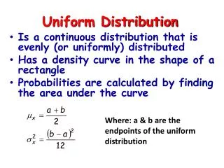
Running-time efficiency • The more “complex” f is, the more time it’s fair to allow. • Fix some measure of “complexity” or “size”, s = s( f ). • Goal: run in time poly(n, 1/, s). • Often focus on fixing s = poly(n), learning in poly(n) time. e.g., size of smallest DNF formula
The “junta” problem • Fits into the formulation (slightly strangely): • is fixed to 0. (Equivalently, 2−k.) • Measure of “size” is 2(# of relevant variables). s = 2k. • [Mossel-O-Servedio ’04] had running time essentially • Even under this extremely conservative notion of “size”, we don’t know how to learn in poly(n) time for s = poly(n).
Assuming factoring is hard, nlog(d) s time is necessary. Even with “queries”. [K ’93] complexity measure s fastest known algorithm depth d circuit size nO(logd-1 s) [LMN ’93, H ’02] DNF size nO(log s) [V ’90] Any algorithm that works in the “Statistical Query” model requires time nk. [BF ’02] Decision Tree size nO(log s) [EH ’89] 2(# of relevant variables) n.704log2s [MOS ’04]
What to do? • 1. Give Learner extra help: • “Queries”: Learner can ask for f(x) for any x.) Can learn DNF in time poly(n, s). [Jackson ’94] • “More structured data”: • Examples are not i.i.d., are generated by a standard random walk. • Examples come in pairs, hx, f(x)i, hx', f(x')i, where x, x' share a > ½ fraction of coordinates. ) Can learn DNF in time poly(n, s). [Bshouty-Mossel-O-Servedio ’05]
What to do? (rest of the talk) • 2. Give up on trying to learn all functions. • Rest of the talk: Focus on just learn monotone functions. • f is monotone , changing a −1 to a +1 in the input can only make f go from −1 to +1, not the reverse • Long history in PAC learning [HM’91, KLV’94, KMP ’94, B’95, BT’96, BCL’98, V’98, SM’00, S’04, JS’05...] • f has DNF size s and is monotone )f has a size s monotone DNF:
Why does monotonicity help? • 1. More structured. • 2. You can identify relevant variables. • Fact: If f is monotone, then f depends on xi iff it has correlation with xi; i.e., E[ f(x)xi] 0. • Proof: If f is monotone, its variables have only nonnegative correlations.
Monotone case complexity measure s fastest known algorithm depth d circuit size any function DNF size poly(n, slog s) [Servedio ’04] Decision Tree size poly(n, s) [O-Servedio ’06] 2(# of relevant variables) poly(n, 2k) = poly(n, s)
Learning Decision Trees • Non-monotone (general) case: • Structural result: Every size s decision tree (# of leaves = s)is -close to a decision tree with depthd := log2(s/). • Proof: Truncate to depth d. Probability any input would use a longer path is · 2−d = /s. There are at most s such paths. Use the union bound. x3 x5 x1 x4 x1 x5 1 x2 +1 1 +1 −1 −1 +1 −1
Learning Decision Trees • Structural result: • Any depth d decision tree can be expressed as a degree d(multilinear) polynomial over R. • Proof: Given a path in the tree, e.g., “x1 = +1, x3 = −1, x6 = +1, output +1”,there is a degree d expression in the variables which is:0 if the path is not followed, path-output if the path is followed. • Now just add these.
Learning Decision Trees • Cor: Every size s decision tree is -close to a degree log(s/) multilinear polynomial. • Least-squares polynomial regression (“Low Degree Algorithm”) • Draw a bunch of data. • Try to fit it to degree d multilinear polynomial over R. • Minimizing L2 error is a linear least-squares problem over nd many variables (the unknown coefficients). • ) learn size s DTs in time poly(nd) = poly(nlog s).
Learning monotone Decision Trees • [O-Servedio ’0?]: • Structural theorem on DTs: For any size s decision tree (not nec. monotone), the sum of the n degree 1 correlations is at most • Easy fact we’ve seen: For monotone functions, variable correlations = variable “influence”. • Theorem of [Friedgut ’96]: If the “total influence” of f is at most t, then f essentially has at most 2O(t) relevant variables. • Folklore “Fourier analysis” fact: If the total influence of f is at most t, then f is close to a degree-O(t) polynomial.
Learning monotone Decision Trees • Conclusion: If f is monotone and has a size s decision tree, then it has essentially only relevant variable and essentially only degree • Algorithm: • Identify the essentially relevant variables (by correlation estimation). • Run the Polynomial Regression algorithm up to degree , but only using those relevant variables. • Total time:
Open problem • Learn monotone DNF under uniform in polynomial time! • A source of help: There is a poly-time algorithm for learning almost all randomly chosen monotone DNF of size up to n3. [Servedio-Jackson ’05] • Structured monotone DNF – monotone DTs – are efficiently learnable. “Typical-looking” monotone DNF are efficiently learnable (at least up to size n3). So… all monotone DTs are efficiently learnable? • I think this problem is great because it is: • a) Possibly tractable. b) Possibly true. c) Interesting to complexity theory people. d) Would close the book on learning monotone fcns under uniform!