Download
1 / 36
480 likes | 967 Vues
Layering, buffering, registering, digitizing…. Peter Fox GIS for Science ERTH 4750 (98271) Week 3, Tuesday, February 7, 2012. Contents. Reading review Assignment 1 Layering Buffering Registering Digitizing Lab on Friday Next class(es). Reading review for last week.

E N D
Layering, buffering, registering, digitizing… Peter Fox GIS for Science ERTH 4750 (98271) Week 3, Tuesday, February 7, 2012
Contents • Reading review • Assignment 1 • Layering • Buffering • Registering • Digitizing • Lab on Friday • Next class(es)
Reading review for last week • MapInfo User Guide and other docs
Layering • Useful for: • Separating contents, structures and developing themes • Implies distinction from other layers?? • MapInfo (and many others) has • A Cosmetic layer • Turn on/ off detail option • AKA Coverage or Level
Layer examples USGS: (L) Shaded-relief map and contour lines generated from the digital elevation model in the study area. (R) The wetlands in the study area ranked according to their vulnerability to pollution on the basis of combination of factors evaluated by GIS
Add a layer • Be as clear as you can about the layer ‘type’ • Points, lines, polygons/ regions • Theme based (e.g. in MapInfo – represented by icons), range, chart, special symbol, grid, raster… • Note also ‘Group Layers’ • Layer Control (from Main menu or Map menu) • Practice on Friday! • User guide, through p.68
Change layer properties • Labels (style, placement), lines, nodes, centroids, etc. • For Cosmetic layer – has restrictions so make sure you read (MapInfo Help system): • Using the Cosmetic Layer • Saving Cosmetic Layer Objects • Saving Objects on the Cosmetic Layer • Removing Cosmetic Objects • Disabling the Save Cosmetic Objects Warning Dialog Box
Reorder layers • Map layers display in the order that they are listed in the Layer Control window, with the bottom layer drawn first and the top layer (always the Cosmetic Layer) drawn last • It is important to order your layers correctly and thus give them some thought or be prepared to experiment! • Hint: Denser information sources typical go on the bottom, lighter ones on top… • Something for Friday – learn how to change the layer order
Layers to improve visibility • E.g. zoom layering – DC street maps, you set the threshold, ~ 5 miles but this depends on your ‘use’
Combining layers • The process of combining and transforming information from different layers is sometimes called map "algebra" insofar as it involves adding and subtracting information (intersect, identity, union, symmetric diff., etc. • Try this on Friday - e.g. open a grid layer, see p.77 (open one of the files downloaded from the /gis/data directory) • Create a new layer of derivative or complementary information • Combine and save…
Buffering • Buffer zone - an area within a given ‘distance’ from a map feature • Points, lines, or polygons can be buffered • Buffers are used to identify areas surrounding geographic features • E.g. to keep septic systems over 100 meters away from streams, locate housing within a quarter mile of existing roads, keep hiking trails away from seasonally flooded rivers, or make sure most of your city is within some maximum distance from a fire station or school
What is produced? • When you buffer on a set of features, the output is a set of polygons. • Buffering points or lines creates a new coverage that is a polygon coverage. • Polygons define an inside and outside region • Inside region = an area less than the specified buffer distance from the feature(s) of interest • Outside region = an area more than the specified buffer distance from the feature(s) of interest
Distances - ~ two types • Fixed – as it implies • E.g. in the two previous examples • Storage of distance is simpler • Variable – buffer distance depends on another attribute of the ‘feature’ (entity) • E.g. in the next example, based on area value, but could be distance from some other entity, or land type, or statutes, or … • Storage of distances is more complex
Inside/ Outside – used for? • These inside and outside regions are typically distinguished by different codes in an attribute table • You should know the specific codes assigned for the software system you use • Why? You may want to label them, color them, establish relations between/ among them, etc.
Registering • Registration consists of specifying the coordinates of a minimum number of points (3) on the image to orient it in geographic space – they are called control points • Three points are needed to determine the axes and scale • You should also try to determine the type of projection used in the original map • Note, this is different from geocoding (we’ll do that next week)
Where from? • Everywhere! • A raster image is a type of computerized image that consists of row after row of tiny dots (pixels) – see last Friday’s class • E.g. you can create a raster image by scanning a paper map • Make sure you store the image in a file that is a supported format • Then, display the file using MapInfo
Formats • There are many different raster image file formats • MapInfo Professional can read the following types of raster image files: JPEG, GIF, TIFF, PCX, BMP, TGA (Targa), and BIL (SPOT satellite), see p. 80
Example – registration points • If you don’t know the projection, you can get the registration by a best-fitting procedure. • In this case you should provide as many registration points as possible.
Sources • Sources of registration points: GPS, other maps, bench marks, geographic data, recognizable points on ground (state boundaries), other spatially enabled data (road vector file) • What are the considerations here? • Scan or download image, or get aerial photo – read into MapInfo as table, register, set up as layer
Overall intent is re-projection! • During a raster re-projection process, the software recalculates the pixel values of the source image to make them display correctly in the destination image. • In this resampling process, the idea is to restore every pixel value of the image based on the pixels around it • MapInfo has two methods for calculating the pixel values of the destination image: • Cubic Convolution • Nearest Neighbor
Example USGS: (L) An elevation image classified from a satellite image of Minnesota exists in a different scale and projection than the lines on the digital file of the State and province boundaries. (R) The elevation image has been re-projected to match the projection and scale of the State and province boundaries.
Iterate, especially now • Get some experience, add/ remove control points • Compare the results from different choices • Should start to give a feel for what are reliable control points (and what are not) • Recall the discussions on what a ‘point’ is and how a line centroid is determined, etc. • Friday!
Digitizing • Your (or with the help of the software) determination of sets of points, lines, etc. on a map in front of you • Also called Heads-up digitizing (versus from a digitizing tablet) • To minimize image distortion, only digitize from map images with known projections or rectified aerial photographs
MapInfo (others similar) • Autotrace - Snap and Trace – Friday! • S-key • T-key (autotrace) • N-key (autonode) • Heads-up – point and click • Practice on simple maps, or simple regions on complex maps • Streaming… • Combining…
Converting • Sometimes (often) you want to convert what you’ve capture into another GIS data type • Polylines to regions - Regions to polylines • E.g. join multiple polylines, split at nodes, • Objects to polylines • E.g. a parcel of land, contains different land-use types • User Guide, pp. 164-165
Summary • Four base topics for GIS (for Science) • Layering • Buffering • Registering • Digitizing • For learning purposes remember: • Demonstrate proficiency in using geospatial applications and tools (commercial and open-source). • Present verbally relational analysis and interpretation of a variety of spatial data on maps. • Demonstrate skill in applying database concepts to build and manipulate a spatial database, SQL, spatial queries, and integration of graphic and tabular data. • Demonstrate intermediate knowledge of geospatial analysis methods and their applications.
Reading for this week • MapInfo Tutorials (esp.) • MapInfo User Guide (also see text book for relevant chapters if available) • Chapter 3 (Basics, esp. Working with Layers in the Layer Control, p. 57) - layering • Chapter 7 (Drawing and Editing Objects, esp. Editing, p. 170) - digitizing • Chapter 10 (Buffering and Working with Objects, p. 268) - buffering • Chapter 12 (Registering Raster Images, p.324) - registering
Friday Feb. 10th • Lab session with Max (I am away) • 12pm-1:30pm (attendance will be taken) • Hands on • Layers • Buffering • Registering • Digitizing • See web page for example data sources to work with
Next classes • Geocoding (encoding) with streets/ addresses • Simple interpolation • Lab on Friday (17th)