Computational Complexity

1. Computational Complexity Jang, HaYoung (hyjang@bi.snu.ac.kr) BioIntelligence Lab.

2. Algorithm Analysis • Why Analysis? • to predict the resources that the algorithm requires, such as computational time, memory, communication bandwidth, or logic gates. • The running time of an algorithm is the number of primitives operations or “step”(machine independent) executed.

3. Complextity • Space / Memory • Time • Count a particular operation • Count number of steps • Asymptotic complexity

4. Time Complexity • Worst-case • an upper bound on the running time for any input • Average-case • We shall assume that all inputs of a given size are equally likely. • Best-case • to get the lower bound

5. Time Complexity • Sequential search in a list of size n • worst-case : n times • best-case : 1 times • average-case :

6. Asymptotic Notation • Asymptotic upper bound, we use -notation. • For a given function g(n), we denote by  (g(n)) the set of functions; (g(n)) = {f(n): there exist positive constants c and n0 such that f(n) <= cg(n) for all n >= n0}.

7. Asymptotic Notation • -notation provides an asymptotic lower bound. • For a given function g(n), we denote by (g(n)) the set of functions (g(n)) = {f(n): there exist positive constants c and n0such that f(n) >= cg(n) for all n >= n0}.

8. Asymptotic Notation • (g(n)) = {f(n) : there exist positive constants c1, c2, and n0 such that c1g(n) <= f(n) <= c2g(n) for all n >= n0}.

9. Asymptotic Notation

10. The sets (n2), (n2), and (n2)

11. Practical Complexities 109 instructions/second computer

12. Impractical Complexities 109 instructions/second computer

13. Faster Computer Vs Better Algorithm Algorithmic improvement more useful than hardware improvement. E.g. 2n to n3

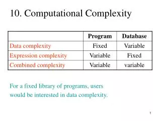
14. Intractability • A polynomial-time algorithm is one whose worst- case time complexity is bounded above by a polynomial function of its input size. • example - worst-case time complexity - Polynomial-time: 2n, 3n3 + 4n, 5n + n10, n log n - Non polynomial-time: • Intractable problem - No polynomial-time algorithm can solve it. W(n)  (p(n))

15. Three Categories of Problems (1) 1. Problems for which polynomial-time algorithms have been found 2. Problems that have been proven to be intractable - The first type is problems that require a non-polynomial amount of output. e.g. Determining all Hamiltonian Circuits. - The second type of intractability occurs when our requests are reasonable and we can prove thattheproblem cannot be solved in polynomial time. e.g. Halting Problem, Presburger Arithmetic Problem

16. Three Categories of Problems (2) Presburger Arithmetic is the theory of integers with addition (Z,+,=,<,0,1) and is known to require doubly exponential nondeterministic time. 3. Problems that have not been proven to be intractable but for which polynomial-time algorithms have never been found e.g. 3-SAT, 0-1 Knapsack, TSP, Sum-of-Subset, Partition, Graph-Coloring, Independent Set, Vertex-Cover, Clique,3D-Matching, Set Cover, etc.

17. The Sets P and NP (1) • Definition P is the set of all decision problems that can be solved in polynomial-time. • A NP algorithm have two stages: 1. Guessing (in nondeterministic polynomial time) Stage 2. Verification (in deterministic polynomial time) Stage • Definition NP is the set of all decision problems that can be solved in nondeterministic polynomial-time.

18. The Sets P and NP (2)

19. Genetic Algorithms

20. An Abstract View of GA generate initial population G(0); evaluate G(0); t := 0 ; repeat t := t + 1; generate G(t) using G(t-1); evaluate G(t); until termination condition has reached;

21. Search Techniques SEARCH TECHNIQUES Calculus-based Guided Random Enumerative techniques. Search Techniques Techniques Dynamic Directed Indirected Simulated Evolutionary Methods Annealing Algorithms PGMing Methods Fibonacci Newton Evolutionary Genetic Algorithms strategies Parallel Sequential GAs GAs Classes of Search techniques

22. Simple Genetic Algo's components 1. A mechanism to encode the solutions as binary strings 2. A population of binary strings 3. A fitness function 4. Genetic operators 5. Selection mechanism 6. Control parameters

23. The GA Cycle Population (chromosomes) Decoded strings Offspring* Crossover & Mutation New Generation Evaluation (fitness) Genetic Operators Parents* Reproduction Manipulation Mates = Evaluation + Selection Selection (mating pool )

24. Fitness function (object function) • The mechanism for evaluating each string • To maintain uniformity over various problem domains, normalize the obj.function to 0 to 1. • The normalized value of the obj. function = the fitness of the string

25. Selection • Models nature's "survival-of-the-fittest " mechanism • A fitter string receives higher number of offspring. • Proportionate selection scheme • The roulette wheel selection scheme

26. Crossover • After Selection, pairs of string are picked at random • If string length = n, randomly choose a number from 1 to n - 1, then use it as a crossover point. • GA invokes crossover ONLY IF a randomly generated no > pc . (pc = the crossover rate)

27. Mutation • After crossover, string are subjected to mutation • Flipping bits : 0 1, 1 0 • Mutation rate : Pm = probability that a bit will be flipped • The bits in a string are independently mutated. = Role : restoring lost genetic material

28. Function Definition Find xfrom the range [-1, 2] which maximizes the f

29. Analysis of function f

30. Representation (1) • Representation of string • six places after decimal point • The range [-1,2] should be divided into at least 3000000 ranges. • Binary representation : 22 bits • Mapping from a binary string into a real number x • Convert the binary string from the base 2 to base 10: • Find a corresponding real number x:

31. Representation (2) String Example : string (1000101110110101000111) String 1111111111111111111111 0000000000000000000000 x 2.0 -1.0

32. Initial Population • Create a population of strings, where each chromosome is a binary vector of 22 bits. • All 22 bits for each string are initialized randomly.

33. Evaluation Function • eval(v) = f(x) • For example, x f(x) Strings f(x1)= 1.586345 f(x2)= 0.078878 f(x3)= 2.250650 x1= 0.637197 x2= -0.958973 x3= 1.627888 v1=(1000101110110101000111) v2=(0000001110000000010000) v3=(1110000000111111000101) The string v3 is the best of the three strings, since its evaluation returns the highest value.

34. v3=(1110000000111111000101) Fifth gene 10th gene v3’=(1110100000111111000101) v3’’=(1110000000011111000101) Genetic Operators : Mutation • Mutation • Mutation alters one or more genes with a probability equal to mutation rate. • Mutation Example :

35. Before Crossover f(x1)= 0.637197 f(x2)= -0.958973 v2=(00000 | 01110000000010000) v3=(11100 | 00000111111000101) x2= -0.958973 x3= 1.627888 After Crossover f(x1’)= 0.940865 f(x2”)= 2.459245 v2’=(00000 | 00000111111000101) v3”=(11100 | 01110000000010000) x2’= -0.998113 x3”= 1.666028 Genetic Operators : Crossover • Crossover Example : • The crossover on v2 and v3 • Assume that the crossover point was randomly selected after 5th gene:

36. Parameters • Population size = 50 • Probability of crossover = 0.25 • Probability of mutation = 0.01

37. Experimental results • The best chromosome after 150 generations • Vmax = (1111001101000100000101) • Xmax= 1.850773 • As expected, , and f(xmax) is slightly larger than 2.85.