Download
1 / 49
490 likes | 526 Vues
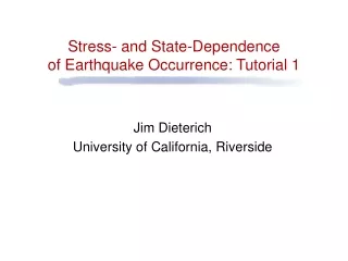
Stress- and State-Dependence of Earthquake Occurrence. Jim Dieterich, UC Riverside. Formulation for earthquake rates. Unified and quantitative framework for analysis of effects of stress changes on earthquake occurrence Some applications: Aftershocks Foreshocks

E N D
Stress- and State-Dependence of Earthquake Occurrence Jim Dieterich, UC Riverside
Formulation for earthquake rates • Unified and quantitative framework for analysis of effects of stress changes on earthquake occurrence • Some applications: • Aftershocks • Foreshocks • Complexity of earthquake events • Triggering of earthquakes by seismic waves • Tidal triggering (why the effect is so weak) • Earthquake probabilities following stress change • Solutions for stress changes from observations of earthquake rates • Stress relaxation by seismic processes for geometrically complex faults
Earthquake rate formulation: Model • Earthquake occurrence is controlled by earthquake nucleation processes • Earthquake nucleation as given by rate- and state-dependent friction is time dependent and highly non-linear in stress and gives the following • Coulomb stress function as where • At steady state • The characteristic time to reach steady-state Dieterich, JGR (1994), Dieterich, Cayol, Okubo, Nature, (2000), Dieterich and others, USGS Professional Paper 1676 (2003)
Earthquake rates following a stress step Earthquake rate (R/r ) Time (t/ta )
Coulomb stress change Earthquake rate Background rate Time Aftershock model Stress Pict of Coulomb change Time
Coulomb stress change Stress Shadow Stress Time Earthquake rate Background rate Time
Method: Stress time series STEPS 1) Select region and magnitude threshold 2) Smooth earthquake rate: R(t) 3) Obtain time series for g: 4) Solve evolution equation for Coulomb stress S. For example:
Figure: Barry Eakins Rift zones modified from Fiske and Jackson (1972) Bathimetry: USGS JAMSTEC
Inversion of EQ rates for stress (1996-1994) Dieterich and others, 2000, Nature
Method to obtain stress changes from earthquake rates 3) Prepare maps (or cross sections) of stress changes over specified time intervals STEPS 1) From earthquake rates obtain time series for gat regular grid points: 2) Solve evolution equation for Coulomb stress S as a function of time at each grid point Dieterich, Cayol, and Okubo, Nature (2000) Dieterich and others, USGS Prof Paper(2003)
1976-1983 >1983 Deformation 0.5MPa/yr (0.1MPa) Seismicity 0.3–0.6 MPa/yr ≤0.1 Mpa/yr Rift intrusion rate 0 .18km3/yr 0 .06km3/yr NS extension 25cm/yr 4cm/yr (Summit region)
0.5 MPa/year Deformation model, 1976-1983 0.2 MPa/year Seismicity solution, 1980-1983 Stress changes before 1983 eruption 2 Dieterich, Cayol, and Okubo, Nature (2000) Dieterich and others, USGS Prof Paper(2003)
Seismicity solution Stress changes at the time of the 1983 intrusion & eruption Deformation model Dieterich and others, USGS Prof Paper(2003)
Stress changes at the time of the 1977 intrusion & eruption Deformation model
M~ 5 Earthquakes following Sept. 13, 1977 eruption M4.6 9/27/79 5.4 9/21/79 M4.6 9/27/79 5.4 9/21/79
M5.0 3/20/83 M5.2 9/9/83 M~ 5 Earthquakes following Jan. 1, 1983 eruption
Geometrically complex faults USGS, 2003
Fault geometry Individual faults exhibit approximately self-similar roughness (fractal dimension~1). Fault in the Monterrey Formation Fault systems also appear to be scale-independent San Francisco Bay Region
Random Fractal Fault Model Solve for slip using boundary elements. Simple Coulomb friction with = 0.6 Periodic B.C, or slip on a patch = 0.3 = 0.1 = 0.03 = 0.01
Slip of a fault patch
Fault slip and stress changes Smooth fault Fractal fault: H=1, =0.01
Global slip Global slip Fault slip and stress changes Smooth fault Fractal fault: H=1, =0.01
Non-linear scaling of slip with fault length Hurst exponent: H = 1.0 Roughness amplitude: = 0.05 Region of ~ linear scaling of Slip with fault length
Non-linear scaling of slip with fault length: Average of slip for n100 simulations dMAX = 85 FAULT LENGTH Hurst exponent: H = 1.0 Roughness amplitude: = 0.1 Region of ~ linear scaling of slip with fault length
= 0.01 = 0.03 = 0.1 = 0.3
Non-linear scaling and system size-dependence Geometric complexity forms barriers to slip. Barrier stress increases with total slip and sequesters strain energy that would otherwise be released in slip. The barrier stress acts as an elastic back-stress, which opposes slip. Back-stress increases linearly with slip. Slip saturates at when the back-stress equals the applied stress. SA = Applied stress Back stress, SBACK Slip, d
= 0.01 = 0.03 = 0.1 = 0.3
Non-linear scaling of slip with fault length Hurst exponent: H = 1.0 Roughness amplitude: = 0.1 Average slip on non-planar faults n~100 Planar fault model with elastic back stress dMAX = 85 FAULT LENGTH
Yielding and Stress Relaxation • Stresses due to heterogeneous slip cannot increase without limit - some form of steady-state yielding and stress relaxation must occur • Slope of 0.01 shear strain .01, brittle failure • In brittle crust, stress relaxation may occur by faulting and seismicity off of the major faults. • Instantaneous failure and slip during earthquake • Post-seismic – aftershocks and long-term seismicity • Yielding will couple to the failure process, by relaxing the back-stresses
Landers and Hector Mine Earthquakes Data from Sowers and others (1992) , US Geological Survey
Steady-state yielding by earthquakes: EQ rate µ Coulomb stress rate µ Long-term slip rate
Earthquake rate Earthquake rate Average long-term earthquake rate by distance from fault with random fractal roughness • Stressing due to fault slip at constant long-term rate • Model assumes steady-state seismicity at the long-term stressing rate, in regions where
Earthquake rate Earthquake rate Average long-term earthquake rate by distance from fault with random fractal roughness Scaling:
Initial Aftershock Rate / Background Rate
Aftershock rates as function of distance 0.01 – 0.03 L 0.03 – 0.05 L 0.05 – 0.07 L 0.07 – 0.09 L 0.09 – 0.10 L L=rupture length
Conclusions: Seismicity stress solutions • Stress shadows are seen for all earthquakes M≥4.7 • Quantitative agreement of deformation measurements and seismicity stress solutions • Stress changes 1976-1983 • Stress changes related to 1983 eruption • Stressing rate change 1980-1983 • Provides greater detail of stress changes at depth than can be obtained from deformation modeling • Resolve stress patterns for earthquakes M~5 at depths of 10km. This includes stress shadows • Useful for guiding deformation modeling, by eliminating alternative models • Reveals stress interactions between magmatic and earthquake processes at Kilauea volcano
Conclusions - Seismicity and non-planar faults • Fault complexity heterogeneous slip and stress • Fault complexity + elasticity non-linear scaling and system size-dependence • Heterogeneous stresses increase with slip yielding & stress relaxation • Slope = 0.01 shear strain .01 brittle failure • Instantaneous failure and slip during earthquake • Fall-off of background seismicity by distance • Post-seismic – aftershocks within “stress shadow” • Stress relaxation process will couple to slip on major faults by relaxing the back stresses. Speculation: • Restore linear scaling • Restore independence of system size