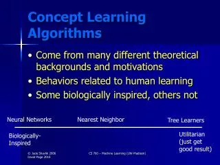
1. Concept Learning Algorithms • Come from many different theoretical backgrounds and motivations • Behaviors related to human learning • Some biologically inspired, others not Neural Networks Nearest Neighbor Tree Learners Utilitarian (just get good result) Biologically- Inspired CS 760 – Machine Learning (UW-Madison)

2. Today’sTopics • Perceptrons • Artificial Neural Networks (ANNs) • Backpropagation • Weight Space CS 760 – Machine Learning (UW-Madison)

3. Connectionism PERCEPTRONS (Rosenblatt 1957) • among earliest work in machine learning • died out in 1960’s (Minsky & Papert book) wij J wik K I L wil Outputi = F(Wij * outputj + Wik * outputk + Wil * outputl ) CS 760 – Machine Learning (UW-Madison)

4. Perceptron as Classifier • Output for N example X is sign(W·X), where sign is -1 or +1 (or use threshold and 0,1) • Candidate Hypotheses: real-valued weight vectors • Training: Update W for each misclassified example X (target class t, predicted o) by: • Wi Wi + h(t-o)Xi • Here h is learning rate parameter CS 760 – Machine Learning (UW-Madison)

5.  E ΔWj - η Wk  E  o  (t – o) = (t – o) = -(t – o) Wk Wk Wk Gradient Descent for the Perceptron(Assume no threshold for now, and start with a common error measure) 2 Error  ½ * ( t – o ) Network’s output Teacher’s answer (a constant wrt the weights) Remember: o = W·X CS 760 – Machine Learning (UW-Madison)

6. Continuation of Derivation (∑k wk * xk)  E Stick in formula for output = -(t – o) Wk Wk = -(t – o) xk SoΔWk = η (t – o) xkThe Perceptron Rule Also known as the delta rule and other names (with small variations in calc.) CS 760 – Machine Learning (UW-Madison)

7. As it looks in your text (processing all data at once)… CS 760 – Machine Learning (UW-Madison)

8. W1X1 + W2X2 = Q X2 = = Q -W1X1 W2 -W1Q W2 W2 X1+ Linear Separability Consider a perceptron, its output is 1If W1X1+W2X2 + … + WnXn > Q 0otherwise In terms of feature space + + + + + + - + -- + + + + - + + -- - + + - - + - -- - - y = mx + b Hence, can only classify examples if a “line” (hyerplane) can separate them CS 760 – Machine Learning (UW-Madison)

9. Perceptron Convergence Theorem(Rosemblatt, 1957) Perceptron  no Hidden Units Ifa set of examples is learnable, the perceptron training rule will eventually find the necessary weights However a perceptron can only learn/represent linearly separable dataset CS 760 – Machine Learning (UW-Madison)

10. Output 0 1 1 0 a) b) c) d) Input 0 0 0 1 1 0 1 1 The (Infamous) XOR Problem Not linearly separable Exclusive OR (XOR) X1 1 b d a c X2 0 1 A NeuralNetwork Solution 1 1 X1 -1 -1 X2 Let Q = 0 for all nodes 1 1 CS 760 – Machine Learning (UW-Madison)

11. The Need for Hidden Units If there is one layer of enough hidden units (possibly 2N for Boolean functions), the input can be recoded (N = number of input units) This recoding allows any mapping to be represented (Minsky & Papert) Question:How to provide an error signal to the interior units? CS 760 – Machine Learning (UW-Madison)

12. A perceptron Hidden Units • One View • Allow a system to create its own internal representation – for which problem solving is easy CS 760 – Machine Learning (UW-Madison)

13. Advantages of Neural Networks Provide best predictive accuracy for some problems Being supplanted by SVM’s? Can represent a rich class of concepts Positive negative Positive Saturday: 40% chance of rain Sunday: 25% chance of rain CS 760 – Machine Learning (UW-Madison)

14. error weight Overview of ANNs Output units Recurrent link Hidden units Input units CS 760 – Machine Learning (UW-Madison)

15. Backpropagation CS 760 – Machine Learning (UW-Madison)

16. E Wi,j Backpropagation • Backpropagation involves a generalization of the perceptron rule • Rumelhart, Parker, and Le Cun (and Bryson & Ho, 1969), Werbos, 1974) independently developed (1985) a technique for determining how to adjust weights of interior (“hidden”) units • Derivation involves partial derivatives (hence, threshold function must be differentiable) error signal CS 760 – Machine Learning (UW-Madison)

17. Weight Space • Given a neural-network layout, the weights are free parameters that define a space • Each point in this Weight Spacespecifies a network • Associated with each point is an error rate, E, over the training data • Backprop performs gradient descent in weight space CS 760 – Machine Learning (UW-Madison)

18. E w Gradient Descent in Weight Space E W1 W1 W2 W2 CS 760 – Machine Learning (UW-Madison)

19. E wN E w0 E w1 E w2 , , , … … … , _ “delta” = change to w w The Gradient-Descent Rule E(w)  [ ] The “gradient” This is a N+1 dimensional vector (i.e., the ‘slope’ in weight space) Since we want to reduce errors, we want to go “down hill” We’ll take a finite step in weight space: E  E w = -  E ( w ) or wi = -  E wi W1 W2 CS 760 – Machine Learning (UW-Madison)

20. “On Line” vs. “Batch” Backprop • Technically, we should look at the error gradient for the entire training set, before taking a step in weight space (“batch” Backprop) • However, as presented, we take a step after each example (“on-line” Backprop) • Much faster convergence • Can reduce overfitting (since on-line Backprop is “noisy” gradient descent) CS 760 – Machine Learning (UW-Madison)

21. E w1 w1 w3 w2 w2 w3 wi w w w “On Line” vs. “Batch” BP (continued) * Note wi,BATCH  wi, ON-LINE, for i > 1 BATCH – add w vectors for every training example, then ‘move’ in weight space. ON-LINE – “move” after each example (aka, stochastic gradient descent) E * Final locations in space need not be the same for BATCH and ON-LINE CS 760 – Machine Learning (UW-Madison)

22. outputi= F(Sweighti,j x outputj) Where F(inputi) = output j 1 1+e bias input -(inputi – biasi) Need Derivatives: Replace Step (Threshold) by Sigmoid Individual units CS 760 – Machine Learning (UW-Madison)

23. 1 1 + e out i = - (  wj,i x outj) Differentiating the Logistic Function F(wgt’ed in) 1/2 F’(wgt’ed in) =out i( 1- out i) 0  Wj x outj CS 760 – Machine Learning (UW-Madison)

24. = (use equation 2) * See Table 4.2 in Mitchell for results = (use equation 3) Error Wi,j Error Wj,k wx,y = -  (E /  wx,y ) BP Calculations k j i Assume one layer of hidden units (std. topology) • Error  ½  ( Teacheri – Outputi ) 2 • = ½ (Teacheri – F([Wi,j x Outputj] )2 • = ½ (Teacheri – F([Wi,j x F(Wj,k x Outputk)]))2 Determine recall CS 760 – Machine Learning (UW-Madison)

25. Derivation in Mitchell CS 760 – Machine Learning (UW-Madison)

26. Some Notation CS 760 – Machine Learning (UW-Madison)

27. By Chain Rule (since Wji influences rest of network only by its influence on Netj)… CS 760 – Machine Learning (UW-Madison)

28. CS 760 – Machine Learning (UW-Madison)

29. Also remember this for later – We’ll call it -δj CS 760 – Machine Learning (UW-Madison)

30. CS 760 – Machine Learning (UW-Madison)

31. Remember netk = wk1 xk1+ … + wkN xkN Remember that oj is xkj: output from j is input to k CS 760 – Machine Learning (UW-Madison)

32. CS 760 – Machine Learning (UW-Madison)

33. outi = F(  wi,j x outj) j Using BP to Train ANN’s • Initiate weights & bias to small random values (eg. in [-0.3, 0.3]) • Randomize order of training examples; for each do: • Propagate activity forward to output units k j i CS 760 – Machine Learning (UW-Madison)

34.  F(neti)  neti F’( netj ) = Using BP to Train ANN’s (continued) • Compute “deviation” for output units • Compute “deviation” for hidden units • Update weights i = F’( neti ) x (Teacheri-outi) j = F’( netj ) x ( wi,j x  i) i • wi,j =  x i x outj • wj,k =  x j x outk CS 760 – Machine Learning (UW-Madison)

35. Using BP to Train ANN’s (continued) • Repeat until training-set error rate small enough (or until tuning-set error rate begins to rise – see later slide) Should use “early stopping” (i.e., minimize error on the tuning set; more details later) • Measure accuracy on test set to estimate generalization (future accuracy) CS 760 – Machine Learning (UW-Madison)

36. Advantages of Neural Networks • Universal representation (provided enough hidden units) • Less greedy than tree learners • In practice, good for problems with numeric inputs and can also handle numeric outputs • PHD: for many years, best protein secondary structure predictor CS 760 – Machine Learning (UW-Madison)

37. Disadvantages • Models not very comprehensible • Long training times • Very sensitive to number of hidden units… as a result, largely being supplanted by SVMs (SVMs take very different approach to getting non-linearity) CS 760 – Machine Learning (UW-Madison)

38. Looking Ahead • Perceptron rule can also be thought of as modifying weights on data points rather than features • Instead of process all data (batch) vs. one-at-a-time, could imagine processing 2 data points at a time, adjusting their relative weights based on their relative errors • This is what Platt’s SMO does (the SVM implementation in Weka) CS 760 – Machine Learning (UW-Madison)

39. Backup Slide to help with Derivative of Sigmoid CS 760 – Machine Learning (UW-Madison)