Download
1 / 12
120 likes | 172 Vues
Learn about constructing the Keynesian Cross, planned vs. actual expenditure, government multipliers, IS curve, loanable funds market, LM curve, and achieving short-run equilibrium in economics.

E N D
The Keynesian Cross Model, The Money Market, and IS/LM Planned expenditure and actual expenditure.
Constructing the Keynesian Cross mpc £1 • Actual expenditure is Y and planned expenditure is E = C + I + G. • I, G, and T are assumed exogenous and fixed. • Our consumption function is C = c(Y–T), where c is the marginal propensity to consume (mpc). • Mapping out E = c(Y–T) + I + G gives us… E Y=E E=C+I+G E* Y Y* • The slope of E is the mpc. • In equilibrium planned expenditure equals total expenditure or Y=E.
Constructing the Keynesian Cross • Equilibrium is at the point where Y = C + I + G. Inventory drops. Inventory accumulates. • If firms were producing at Y1 then Y > E E Y=E • Because actual expenditure exceeds planned expenditure, inventory accumulates, stimulating a reduction in production. E=C+I+G E* mpc • Similarly at Y2, Y < E £1 • Because planned expenditure exceeds actual expenditure, inventory drops, stimulating an increase in production. Y Y2 Y* Y1
Government expenditure and tax multipliers E2 E3 Y3 Y2 • An increase of G by ΔG causes an upward shift of planned expenditure by ΔG. • Notice that ΔY > ΔG. This is because although ΔG causes an initial change in Y of ΔG, the increased Y leads to an increase in consumption and triggers a multiplier effect. E Y=E ΔG • Now suppose a decrease of T by ΔT that causes an upward shift of planned expenditure by mpc*ΔT. mpc*ΔT E1 • Notice again that ΔY > ΔT but that ΔY is less than in the case with ΔG. This is because ΔT causes no initial change in Y as ΔG did, the decrease in T simply leads to an increase in consumption and triggers the multiplier effect. Y Y1
Building the IS curve E Y r r I Y E=Y • The IS curve maps the relationship between r and Y for the goods market. Let the interest rate increase from r1 to r2 reduce planned investment from I(r1) to I(r2). E=C+I(r1)+G This decrease in investment causes the planned expenditure function to shift down. So Y decreases from Y1 to Y2. The IS curve maps out this relationship between the interest rate, r, and output (or income) Y. E=C+I(r2)+G ΔI Y2 Y1 r2 r2 r1 r1 IS I(r) Y2 Y1 I(r2) I(r1)
Shifting the IS curve E Y r Y E=Y • While changing r allows us to map out the IS curve, changes in G, T, or mpc cause Y to change for any level of r. This causes a shift in the IS curve. E=C+I+G2 E=C+I+G1 ΔG Suppose an increase in G causes planned expenditure to shift up by ΔG. Y1 Y2 For any r the increase in G causes an increase in Y of ΔG times the government expenditure multiplier. r1 Therefore, the IS curve shifts to the right by this amount. IS´ IS Y1 Y2
A loanable funds market interpretation r r I Y • The IS curve maps the relationship between r and Y for the loanable funds market in equilibrium. • Suppose Y increases from Y1 to Y2. This raises savings from S(Y1) to S(Y2) resulting in a lower equilibrium interest rate. • The IS curve maps out this relationship between the lower interest rate and increased income. S(Y1) S(Y2) r1 r1 r2 r2 IS I(r) Y1 Y2
A loanable funds market interpretation of fiscal policy r r r2 I Y • While changing r allows us to map out the IS curve, changes in G, T, or mpc cause Y to change for any level of r. This causes a shift in the IS curve. • Suppose again an increase in G. In the loanable funds market this results in a decrease in S and an increase in the interest rate. • Therefore, for a given Y there is a higher level of r. So, the IS curve shifts up by this amount. S(G2) S(G1) r2 IS´ r1 r1 IS I(r) Y1
Building the LM curve r r LM r2 r1 r1 Real Money Balances Y Y1 Y2 • The LM curve maps the relationship between r and Y for the money market. Given money supply and money demand suppose an increase in income raises money demand. The LM curve maps out this relationship between r and Y. (M/P)s r2 L(r,Y1) L(r,Y2)
Shifting the LM curve r r (M2/P)s (M1/P)s r1 r1 L(r,Y) Real Money Balances Y Given money supply and money demand suppose a decrease in the money stock shifts real money supply to the left resulting in a higher equilibrium interest rate. • While changing money demand allows us to map out the LM curve, changes in M or P cause r to change for any level of Y. This causes a shift in the LM curve. Now there is a higher real interest rate for the current level of output. The LM curve shifts up so that at the same level of output the interest rate is higher. LM´ LM r2 r2 Y
IS=LM: The Short Run Equilibrium r LM Y • Given our IS and LM equation we can now determine the short run equilibrium interest rate and output • By mapping out the relationship between Y and r when the goods market (or loanable funds market) is in equilibrium we get the IS curve. • By mapping out the relationship between Y and r when the money market is in equilibrium we get the LM curve. • When we set IS=LM we can solve for the equilibrium levels of r and Y. This represents simultaneous equilibrium in the goods market (or loanable funds market) and the money market. r* IS Y*
Conclusion • We constructed the IS curve from the goods market and from the loanable funds market. We discussed shifting factors for IS. • We constructed the LM curve from the money market and discussed shifting factors for LM. • Finally, we set IS=LM to achieve equilibrium in all markets giving us short run equilibrium r and Y.