Download
1 / 49
500 likes | 652 Vues
Benefit Cost Analysis (BCA) Overview and introduction to discounting. CHRIS MADDEN , www.grinningplanet.com. Environmental regulation involves tradeoffs between environmental quality vs. the costs of regulation. “….we’re getting rid of the ones that kill jobs.”.

E N D
Benefit Cost Analysis (BCA) Overview and introduction to discounting CHRIS MADDEN, www.grinningplanet.com
Environmental regulation involves tradeoffs between environmental quality vs. the costs of regulation “….we’re getting rid of the ones that kill jobs.”
Basic BCA literacy can help you spot (and avoid) instances of economic idiocy
Rise of BCA was in part a reaction to the growing size of regulations • growing impact of regulations on the economy (> $200B/yr [1996]) need for reform need for economic analysis BCA • “…former presidents Carter, Reagan, and Bush and President Clinton have all introduced formal processes for reviewing economic implications of major environmental, health, and safety regulations.” (Arrow et. al, 1996)
Federal approach to BCA is codified in executive orders and OMB docs • “direct(s) federal agencies to perform a…BCA…for economically significant rules” >$100M annual effect on the economy • “OMB’s Circular A-4 (2003) provides guidance to federal agencies on the development of regulatory analysis of economically significant rules as required by EO 12866.” (EPA Guidelines, 2010)
BCA Roadmap • Overview: theoretical foundations & steps • Aggregating over time: discounting • Uncertainty and risk • Politics and the role of BCA: usefulness, impact and criticisms Future lectures/discussions: • Valuation of the environment (“the benefits”) • Measuring the costs of regulation • Application: Arsenic in drinking water. • Climate change
Overview • BCA: estimating the net benefits of a particular action/policy by estimating the costs and benefits, usually (but not always) with the goal of comparing multiple alternatives on the criteria of (Kaldor-Hicks)efficiency • Sometimes also used to inform questions of equity by differentiating net benefits by group • Usually cast in monetary terms
The 1985 EPA Regulatory Impact Analysis of Lead in gasoline seen as a “Cadillac” example of BCA • Policy evaluated: sharp reduction of lead in gasoline • Described in K&O p. 44-45 • Issue: significant research linking lead in blood to • health and learning ability problems in children • premature adult mortality from hypertension • Note on approach: Benefits and costs measured as incremental changes relative to the baseline (conforming to the decision faced). • NOT an attempt to measure the full value of the environment.
Farrow and Toman (1999) (valve seats of older engines) (e.g. some chronic health effects) B2 < B3 (annual)
The are common steps and best practices in BCA (Farrow and Toman, 1999)
When policies involve a streams benefits & costs over time we must decide what relative weight to put on the future
Discounting is a method for placing weights on future values to convert them into present values so that they can be combined to a single number in common units, the “present value”. time t1 t2 0 (present)
The weight placed on a future payoff is determined by the discount rate and # of years until payoff. • discount rate, r: • a parameter that determines the discounting factor or weight, dt • typically: zero to 10% • discounting factor, dt: • the weight placed on a value accrued in year t to convert it to a present value in the present (year 0). • typically <1
Rationale 1: We should discount to account for the opportunity cost of investment. • Public (environmental) sector investments should generate returns at or above the level available in the private sector. • E.g. business loan interest rate, rate of return in the stock market • “Time value of money”, “opportunity cost of capital”
Rationale 2: We should discount because it is consistent with how individuals make decisions in the face of tradeoffs over time. • Individuals are “impatient”. • Individuals are typically indifferent between payoff X at time t and payoff Y<X at time t’ < t. • E.g., I will give you $100 in 1 year: What would you be willing to accept today in lieu of this promise? • Jargon: “pure rate of time preference”
A common approach to choosing a social discount rate is to estimate the observed return to investment (long-run, after-tax, risk-free) • 7%: approx. the real return to investment in large companies (1926–1990) (Newell and Pizer, 2004) • But personal taxes (up to 50%) mean that return to investors, the consumption rate of interest, is closer to 4%. • And this 4% return includes a premium for risk (firms may fail). • To separate the issue of risk from this analysis, consider relatively safe government bonds: 4% nominal return2% after taxes. • “The appropriate rate …. in the United States is generally taken to be around a 3% real, riskless rate.” (Kopp et. al, 1997)
Note: Real versus nominal • Discount rates are NOT meant to address inflation (before discounting all values should be in real terms). • Nominal value: expressed in the money of the day • Real value: adjusted for inflation • In a BCA analysis, benefits and costs from each year are stated in the same real units, e.g. in 2012 dollars.
Discount rates have strong implications for environmental investment/dis-investment Higher discount rates: • favor more rapid depletion of nonrenewables and lower stock levels of renewables (Conrad, J.M. Resource Economics. 1999.) • can make investments to improve environmental quality relatively less attractive compared to those in the private sector (Conrad, J.M. Resource Economics. 1999.)
Higher discount rates don’t favor investments (e.g. in env. quality) when they follow a typical profile • increase the probability of a negative PVNB for projects with high immediate costs and delayed benefits (typical feature of investments in environmental quality—recall Excel demo) • r = 6% 4% • almost doubles the estimate of the MB from CO2 emission reductions (Pearce et al. 2003) • r = 4% declining discount rate approach • nearly doubles the estimate again (Weitzman, 2001)
PVNB calculation example Goulder and Stavins (2002) “An eye on the future” • Simplified climate policy question Should we implement a GHG control policy with • Immediate cost: $4B • One-time benefit in 100 years: $800B • Discount rate: 5% • What’s the PVNB?
t=1 t=16 ∞ • Example D: What is the PVNB given a discount rate, r = 0.05 and: • NBt = 6, t = 1,…,15 and then NBt = 20, t = 16,…,∞. PVNBt=1:15 PVNBt=16:∞ t=1 t=16 t=1 t=16 ∞ ∞ PVNBt=16:∞ t=1 t=16 ∞ PVNBt=1:∞ = PVNBt=1:15 + PVNBt=16:∞
Alternative decision criteria for long-run policy questions • Efficiency: What option provides the greatest PVNB (if question is go/no-go, is the PVNB > 0)? 2. Alternative: responsibility under considerations of intergenerational equity (distribution) • We should judge intergenerational fairness by direct examination (not via an artificially deflated discount rate).
Federal guidelines • U.S. OMB 2003 : • provide estimates of PVNB using discount rates of 3% and 7% • 3%: consumption rate of interest (i.e. after tax return on investments) • 7%: OMB estimate of the opportunity cost of capital • see: http://www.whitehouse.gov/omb/circulars_a004_a-4/ • “Many economists believe that this…range…is too high” (Fraas and Lutter, 2011)
There is no consensus on a single value for the social discount rate Q: What discount rate do you favor for discounting long-term environmental projects? Respondents-over 2,000 Ph.D. level economists Weitzman, M. L. (2001). “Gamma discounting.” American Economic Review 91, 260-271. Image: http://www.dbj.jp/ricf/en/research/symposium199511.html
There is no consensus on a single value for the social discount rate Weitzman (2001): “The most critical single problem with discounting future benefits and costs is that no consensus now exists, or for that matter has ever existed, about what actual rate of interest to use.” The considerations on which a discount rates are based “are fundamentally matters of judgment or opinion, on which fully informed and fully rational individuals might be expected to differ.”
Caveats • “We should have less confidence in a project for which • the sign of the PVNB is highly sensitive to • the discount rate or to • small changes in projected future benefits and costs, compared with a project with a PVNB that is not very sensitive to these elements.” (Goulder and Stavins 2002, p. 674)
Caveats II • The justification for a pure rate of time preference is based on the choices individuals make about payoffs in their own lifetime. • Some economists argue that at the societal level there is no good ethical argument for using a pure rate of time preference other than zero. • Especially, across generations.
Summary of theoretical foundations of BCA Basics: • Benefits: increases in human well-being (utility). • Costs: reductions in human well-being. • For a project or policy to qualify on cost-benefit grounds: • Versus the status quo: its social benefits must exceed its social costs (NB>0). • Versus a set of alternatives: it must have the highest net benefits (be most efficient) (Pearce et al. 2006, Ch. 2)
Summary of theoretical foundations of BCA Scope and aggregation • “Society” is simply the aggregation of individuals. • Geographical boundary: often national (but can be local or int’l) • Aggregating benefits across different social groups or nations can involve summing willingness to pay/accept (WTP, WTA), either 1. regardless of the circumstances of the beneficiaries or losers OR 2. with higher weights to disadvantaged or low income groups • [Rationale: marginal utilities of income will vary, being higher for the low income group] (Pearce et al. 2006, Ch. 2)
Summary of theoretical foundations of BCA • Time • Aggregating over time involves discounting • Establishing the weight placed on future benefits and costs relative to today • Discounted future benefits and costs are known as “present values” • Inflation should be netted out to secure constant price estimates. • Valuation • The notions of WTP and WTA are firmly grounded in the theory of welfare economics • (Correspond to economic notions of compensating and equivalent variations) • WTP and WTA can diverge, sometimes substantially, and with WTA > WTP. (Pearce et al. 2006, Ch. 2)
Politics and the role of BCA: usefulness, impact and criticisms
The devil’s in the details "….benefit-cost analysis has a solid methodological footing and provides a valuable performance measure for an important governmental function, improving the well-being of society. ... However, benefit-cost analysis requires analyticaljudgments which, if done poorly, can obfuscate an issue or worse, provide a refuge for scoundrels in the policy debate.“ Farrow and Toman (1999)
Consensus view of economists on BCA: Exceptionally useful, but not sufficient “Although …benefit–cost analysis • should not be viewed as either necessary or sufficient for …public policy, • it can provide an exceptionally usefulframework for • consistently organizing disparate information, • …greatly improve the process and, hence, the outcome of policy analysis.” Arrow KJ, Cropper ML, Eads GC, Hahn RW, Lave LB, Noll RG, Portney PR, Russell M, Schmalensee R, Smith VK, et al. Is there a role for benefit-cost analysis in environmental, health, and safety regulation? Science 272:221-222 (1996).
How BCA can improve policy Hahn & Dudley (2007) • Stokey and Zeckhauser (1978) & Raiffa (1970) • Efficiency: help decision makers select policies with positive net social benefits • Equity: identify the likely winners and losers as a result of a policy • Uncertainty: evaluate the impact of uncertainty on the net benefits of different policies, • Learning: assess the potential value of new information • Viscusi and Hamilton (1999) • Ignorance: can also help identify key deficiencies in our understanding • Sensitivity: show how sensitive the results are to different assumptions
Benefit-Cost Analysis"How to Lie with Benefit-Cost Analysis” • Fiddle with the definition of baselines so that benefits of regulation are enlarged or costs are diminished (e.g. 2008 lead standard) • Omit impacts or costs that do not support your cause • Use upper- or lower-bound estimates of benefits or costs. • Omit alternatives that you don't wish to see implemented. • Limit the monetization of benefits to make it difficult to compare benefits to costs. • Use discounting assumptions that distort benefits or costs.
Criticism: theoretical foundations • The extent to which CBA rests on robust theoretical foundations as portrayed by the Kaldor-Hicks compensation test. • The fact that the underlying “social welfare function” in CBA is one of an arbitrarily large number of such functions on which consensus is unlikely to be achieved. • The extent to which one can make an ethical case for letting individuals’ preferences be the (main) determining factor in guiding social decision rules. (Pearce et al. 2006, Ch. 2)
Uncertainty • Uncertainty: future outcomes are not know with certainty (they are not “deterministic”) • Risk: probability measure is known (can be crude). • E.g. if outcome is determined by flipping a coin, we know the probability of “heads” • Ambiguity: probability measure is unknown. • E.g. …don’t know the true probability of heads, or even if the process is like flipping a coin.
Expected value • What number do we use for BCA when we don’t know exactly what will happen (i.e. under uncertainty)? • Expected value (aka “mean”) of a random variable: • The integral of the random variable with respect to its probability measure. • Discrete random variables: • the probability-weighted sum of the possible values. • If we were to observe an infinite sequence of independent draws of the random variable, the average should converge to the expected value. • Possible confusion • NOT the mode (most probable value). • “Value” in “expected value” doesn’t refer to “economic” or “monetary” value. Ross (2007), Hamming (1991)
Working with uncertainty: Expected value • Expected value of a “random variable” • A cheerful example: • Let X represent the annual number of deaths that occur from a hazardous chemical at a landfill. Ahead of time this number is unknown. • E(X) = the expected value of X = the sum of each possible value X can take, weighted by the probability it will occur = X1*Pr(X1) + X2*Pr(X2) + …. + XN*Pr(XN) , Pr(Xi) , Xi X1 = X2 = . . XN=X5= 0.27
Expected value: Who wants to be a millionaire?! • Suppose you’ve already won $64K. • You are facing a tough question for $125K. • Your choices • 1) Quit and walk away with $64K • 2) Try to answer the question. If you get it right you win $125K; if you get it wrong you get $0. • What is the best choice? • What option provides the greatest “expected value of NB” or ENB? $125K h/t: Shuzo Takahashi, UND
Expected value: Who wants to be a millionaire?! • What are the ENB (expected net ben.) of your two choices? • 1) Quit and walk away with $64K ENB(quit) = 1*64 = 64 (only 1 possibility) • 2) Try to answer the question. If you get it right you win $125K; if you get it wrong you get $0. ENB(answer) = Pr(correct)*125 + Pr(wrong)*0 $125K • Suppose Pr(correct) = 0.52. Pr(wrong) = 1-Pr(correct) = 0.48. • Then ENB(answer) = 0.52*125 + 0.48 *0 • = $65K $65K=ENB(answer) > ENB(quit)=$64K h/t: Shuzo Takahashi, UND
Federal guidance in A-4 • “Your analysis should provide sufficient information for decision makers to grasp the degree of scientific uncertainty and the robustness of estimated probabilities, benefits, and costs to changes in key assumptions” (U.S. OMB 2003, p. 40). • because of the potential compounding of high-end or low-end assumptions in developing benefits estimates, the analyst, decision makers, and the public cannot know without a quantitative uncertainty analysis whether the estimates provided by an RIA are within the ballpark of likely effects • “…virtually no (regulatory impact analyses) provided a full characterization of uncertainty” (Fraas and Lutter, 2011).
Uncertainty and decision-making • Descriptive (“positive”) application: NRC (Chp. 6, 2004) • Under deterministic outcomes: individuals seek to maximize their utility • Under uncertainty: maximize their expected utility • A sum of utility at each possible outcome weighted by the probability that outcome will occur • Prescriptive (“normative”) application • Advocate decision which maximizes expected utility or expected net benefits.
Estimating a social discount rateOption 2: Ramsey Framework Ramsey (1928) optimal growth model equation: Economy operates as if a “representative agent” selects consumption and savings to max NPV of the stream of utility from consumption over time. • r = ρ + ƞg • r: real return to capital, long-run equilibrium • ρ: pure rate of time preference “time discount rate”, due to “impatience” • ƞ: elasticity of marginal utility w.r.t. consumption • g: average growth in consumption per capita
Estimating a social discount rateOption 2: Ramsey Framework • r: real return to capital, long-run equilibrium; ρ: pure rate of time preference; ƞ: elasticity of marginal utility w.r.t. consumption; g: average growth in consumption per capita • Descriptive approach/Nordhaus & the DICE model • Use economic data to estimate parameters: • Nordhaus (2008): • r = ρ + ƞg = 0.04 (average over the next century (Nordhaus, 2008, 10)) • 5.5% over first 50 years (61). • Economic growth and population growth will slow, rate will fall over time. • Prescriptive approach/Stern & the Stern Review (2006) • Argument: No ethical reason to discount future generations due to a pure rate of time preference except for the possibility that we might not be here at all (ρ reflects only ann. prob. of extinction). 1.3% growth assumed. • r = ρ + ƞg = 0.001 + 1*0.013 = 0.014