Download
1 / 40
400 likes | 549 Vues
Mass and Spin from a Sequential Decay with a Jet and Two Leptons. Michael Burns University of Florida Advisor: Konstantin Matchev Collaborators: KC Kong, Myeonghun Park. Contents. New Physics and Sequential Decays Mass Determination Kinematical Endpoint Method

E N D
Mass and Spin from a Sequential Decay with a Jet and Two Leptons Michael Burns University of Florida Advisor: Konstantin Matchev Collaborators: KC Kong, Myeonghun Park
Contents • New Physics and Sequential Decays • Mass Determination • Kinematical Endpoint Method • Kinematical Boundaryline Method • Spin Determination • Chiral Projections • Basis Functions • Reparametrization
“old” physics: “new” physics, “DCBA”: New Physics and Sequential Decays • At LHC: colored particle production (j), unknown energy and longitudinal momentum (D) • Assume OSSF leptons (ln, lf), missing transverse momentum (A) • What is the new physics (assuming the chain “DCBA”)? • What are the masses of A,B,C,D? • What are their spins?
Method of Kinematical Endpoints (arXiv:hep-ph/9907518, Figs. 1 and 4) Use extreme kinematical values of invariant mass. (“model-independent”) These values depend on spectrum of A,B,C,D … … however, the dependence is piecewise-defined. Offshell B: Njl = 4 (e.g. JHEP09(2000)004 and JHEP12(2004)003)
Inversion and Duplication These inversion formulas use the jll threshold! • Experimental ambiguity • Finite statistics, resolution -> “border effect” • Background -> “dangerous feet/drops” • Piecewise defintions: hmm… largely ignored • Inversion formulae depend on unknown spectrum • Ambiguity DOES occur! picture of a foot, just for fun
Appendix: Example Duplication Change columns to “Njl” How to resolve? We have a technique.
Two Variable Distribution: ---------- MAIN POINT: shapes of kinematical boundaries reveal Region => no more piecewise ambiguity (from perfect experiment). Njl = 3 Njl = 4 Njl = 2 Njl = 1
easy to see restricted ( ) distribution Two Variable Distribution: -------- We know the expression for the hyperbola.
Spin Assignments Assume q/qbar jet S = scalar F = spinor V = vector Each vertex changes spin by (+/-)1/2
Spins and Chiral Projections IJ=11 IJ=12 IJ=22 IJ=21 Four helicity groupings, depending on RELATIVE (physical) helicities of the jet and two leptons. -> four “basis functions” I: relative helicity b/w j and ln J: relative helicity b/w ln and lf spin of antifermion is “opposite of the spinor”?
“Near-type” Distributions I will change mass-ratio coefficients to generic (no one cares). etc. The arrow subscripts indicate the relative helicities. BOTH HELICITY COMBINATIONS CONTRIBUTE! (Notice what happens for equal helicity contributions.) (“near-type” applies in SM: top decay)
“Near-type” Distributions Show plots?
Observable Spin Distributions “cleverly” redefine spin basis functions (like change of basis) Relevant coefficients are the following combinations of couplings: Distribution decomposed into model-dependent (a, b, g) and model-independent (d) contribution etc. I will rewrite this, slightly simpler.
Observable Spin Distributions Dilepton: purely “near-type” (nice) Only one model-dependent parameter (for each spin case): a !!! Get as much use out of this one as possible (as usual). Jet-lepton: must include “near-type” and “far-type” together, piecewise defined D gives charge assymtery; fits to independent model parameters b and g S fits to same a as L !!! extra constraint So, in addition to spin, get three measurements of the couplings through a, b, g – extra model determination.
Dbg La Sa Example: SPS1a We generated “data” from DCBA = SFSF, assuming The fits were determined by minimizing:
Other Spin Assignments Dbg seems the most promising to discriminate the SPS1a model. However, the most discriminating distribution depends on the masses and spins of the true model. Some models cannot even be discriminated, in principle (using our method). (This does not imply that our method is bad; just general.)
Summary • Mass determination: • We have inversion formulas using jll threshhold. • We identified the ambiguous endpoint Regions. • We devised the kinematical boundaryline method, which resolves the ambiguity (ideally). • Spin determination: • We devised a method that allows the model-dependent parameters to float. • We found a convenient spin basis for these floating parameters. • We identified the problem scenarios (fakers).
Appendix: tree-level production • Assuming extra conserved quantum number and 2 to 2 production: • SM in s-channel • Gluon (SU(3) => dominant?) • Electroweak • Higgs (Yukawa => suppressed by SM vertex?) • BSM in t-channel • New color octet (e.g. gluino, KK gluon?) • New color triplet (e.g. squark, KK quark?) • New color singlet (e.g. gaugino, KK photon?) Draw some diagrams.
Appendix: Backgrounds • SM • ISR, Z->dilepton, tau->lepton • Other BSM • Multiple resonances, alternative processes • Combinatoric • Which lepton? Which jet? Draw some diagrams.
Appendix: OF Subtraction (leptons) desired signal: chi20 - chi10 = 68 GeV event selection: 2 OSSF leptons and four “pT-hard” jets (ATLAS TDR 1999 Figs. 20-9 and 20-10) (Hinchliffe, Paige, Shapiro, Soderqvist, Yao, LBNL-39412, Figs. 15 and 16) basically same as above
Appendix: ME Subtraction (jets) jet+lepton distribution desired signal: (different from ours) squark - sneutrino = 284 GeV event selection: one lepton and two “pT-hard” jets (Nurcan Ozturk (for ATLAS), arXiv:0710.4546v2, Fig. 2)
in (.,1) Appendix: Regions & Configurations in rest-frame of C: (1,.) and (5,.) (2,.) (3,.) (4,.) and (6,.) independently of frame: in rest-frame of B:
Background Background Appendix: Dangerous Feet/Drops (arXiv:hep-ph/0510356, Fig. 10)
For Njl = 1,2,3 Appendix: HiLo Points
Appendix: 2D hi vs lo Distribtuions for Duplicated Points Maybe zoom in to pdf before copying to show points?
Appendix: 2D jll vs. ll Distribtuions for Duplicated Points Maybe zoom in to pdf before copying to show points?
Appendix: Chirality vs. Helicity What to say? (It still confuses me.)
Appendix: particle/antiparticle fraction ??? ??? I have to find a reference.
Appendix: “Near-type” Basics C’B’A’ = { SFS , SFV , FSF , FVF , VFS , VFV } One of either I or J is irrelevant. C’B’A’fbfa = { CBAlnlf , DCBjln }. Only the relative helicity between fa and fb is important. Chiral projections allow helicities to be selected by the couplings (because f’s are massless), so that matrix element can be spin-summed. • Spin dependence requires either: • chiral imbalance (gL/=gR) at both vertices, or • B’=V.
Appendix: “Near-type” Width Show basic calculations: Spin sums and contractions, Narrow width approximation,
Appendix: “Near-type” with Clebsch-Gordan Show basic calculations: Clebsch-Gordan Coefficients
Appendix: the “far-type” log behavior Whereas the “near-type” distributions are polynomials in m2, the “far-type” distributions (not presented), in addition to being more complicated, generally have some logarithmic m2-dependence. This can actually be easily “motivated”. Show near vs. far. Show Jacobian stuff.
Appendix: Fakers FSFV always fakes FSFS. FSFS can also fake FSFV for some mass spectra. The only condition is: I just need to fill this in (also for FVFS/FVFV). Maybe I will show the plots for FSFV data.