MacLennan
MacLennan. Chapter 1 The Beginning: Pseudo-code Interpreters. History and Motivation. Programming is difficult. Because of its complexity, dealing with many different details at one time. Programming early computers was especially difficult.

MacLennan
E N D
Presentation Transcript
MacLennan Chapter 1 The Beginning: Pseudo-code Interpreters
History and Motivation • Programming is difficult. • Because of its complexity, dealing with many different details at one time. • Programming early computers was especially difficult. • Very little storage, slow, complicated programming • Four address, optimal coding, drum head • Irregular and hardware based op codes • Many program design notations were developed.
Floating point and indexing were simulated. • It was very difficult. • Development of floating-point subroutines: slow but simple • Pseudo-code Interpreters were invented. • Pseudo-code Interpreters implemented a Virtual computer with its own set of data types(floating point) and operations(indexing) in terms of the real computer with its own data types and operations.
The Automation Principle Automate mechanical, tedious, or error prone activities. • The virtual computer is in a higher level than the real one. • Provide more suitable facilities. • Eliminate many details.
The Regularity Principle Regular rules, without exceptions, are easier to learn, use, describe, and implement. • The virtual computer is more regular than the real one. • Simpler to understand through the absence of special cases.
All programming languages can be viewed as defining virtual computers. • Better in some respects • Usually slower
Compiling Routines • Extract subroutines from libraries and combine them (compiling). • Less overhead, is done once. • Will be discussed in following chapter.
Design of a Pseudo-code • Similar to real pseudo-codes, languages L1 and L2, Bell Labs, for the IBM 650, in 1955 and 1956. • Goal: Illustrating many of the steps and decisions in design of a programming language.
Assumptions and Facilities • A computer with 2000 words of 10-digit memory • We want facilities as: • Arithmetic • Control of execution flow • Input-output
Functions • Floating-point arithmetic • Floating-point comparisons • Indexing • Transfer of control • Input-output
Make a decision • How large shall the addresses be? • Two, three, or four? • Two: 100 locations • Three: 1000 locations • Four: 10,000 locations
Three digits: • Addressing only 1000 locations security • First 1000 locations for data • We are unable to address out of data area
The Impossible Error Principle Making errors impossible to commit is preferable to detecting them after their commission. • With our addressing rule, we prevent the programmer to overwrite program or the interpreter.
Next decision • The instructions could have two, three, or four operands. • Two addresses: x+y x • Three addresses: x+y z • Four addresses: x+y*z w
Instructions have three operands. • Encoding of 20 operations is possible op opn1 opn2 dest +1 010 150 200 add …
The Orthogonality Principle Independent functions should be controlled by independent mechanisms. • A corollary of regularity principle. • Wecan describe m*n different possibilities even though we only have to memorize m+n independent facts.
Design Principles must be applied flexibly • Some of the principles contradict one another. • A balance must be find. • No rules for this balancing task • Experience gives you a good eye!
Orthogonality may be inappropriate • Some of m*n possibilities may be: • Useless • Difficult to implement • Illegal Remember these as exceptions.
+4 200 201 035 • If [200] = [201] then goto 035 • Data location 200,201 • Program location 035 • -5 702 000 100 • If [702] < 0 then goto 100
Moving • Do we need a ‘moving operation’? • +1 150 000 280 • [150] [280] • But this is slow!
Moving • +0 for move • (why +0 and not +6 ?) • Easy-to-remember series of operations: • Move, add, multiply, square (increasing complexity) • Application of Regularity Principle
Indexing and Loops • We need • Address of the array • Address of the index variable • So, we used two of the three address fields in the instruction.
What operation(s) shall we define on arrays? • Move them to or from other locations • +6 xxx iii zzz xi z • -6 xxx yyy iii x yi
Examples for indexing • We have a 100-element array beginning at location 250 in data memory, and location 050 contains 17, • +6 250 050 803 • Move [267] to 803 • -6 722 250 050 • Move [722] to 267
Loops • Initialize, increment, and test index variables • We can use instructions which already exist, but • They are floating point operations • Indexing is used very often
The Abstraction Principle Avoid requiring something to be stated more than once; factor out the recurring pattern. • It is a corollary of Automation Principle. • Results to the appearance of modules.
+7 for increment and test indices • We need to know • The location of the index • The location of the upper bound for the loop • The location where the loop begins
+7 iii nnn ddd • iii : address of the index, • nnn : address of the upper bound, • ddd : location of the beginning of the loop • [iii]+ +; if [iii] < [nnn] then go to ddd;
Input-Output • +8 • Read a card containing one 10-digit number into a specified memory location. • -8 • Print the contents of a memory location
Pseudo-Code operations table Page 19
Program Structure • How do we arrange to get the program loaded into memory? • How do we initialize locations in the data memory? • How do we provide input data for the program?
Program Structure Initial data values (Declarations) +9999999999 Program instructions (executable statements) +9999999999 Input data
Implementation • Automatic Execution is patterned after manual execution • Iterative interpreter • Recursive interpreter
The read-execute cycle is the heart of an iterative interpreter • Read the next instruction. • Decode the instruction. • Execute the operation. • Continue from step 1 with the next instruction.
Where shall we add IP := IP + 1 ?
Interpreters simplify debugging. • Add an instruction to the interpreter to get a trace of the execution of the program. • Statement labels simplify coding. • Using absolute locations in pseudo-code instruction, make changes error-prone and tedious.
The Labeling Principle • Do not require the user to know the absolute position of an item in a list. Instead, associate labels with any position that must be referenced elsewhere.
Label definition operator • -7 0LL 000 000 • It is a non-executable statement. • It is a declaration and say bind a symbolic label to an absolute location. • So we will have: +4 xxx yyy 0LL , • Look at page 27
How can we interpret labels? • Label tables • We have to know • all the labels are defined once, • if there is any referencing to undefined labels, • if a label is defined in more than one place.
Variables can be processed like labels • We can have variable declarations in Initial-data section of the program: • +0 sss nnn 000 • d ddd ddd ddd • Declare a storage area with symbolic name sss, nnn locations long, initialized to all d ddd ddd ddd
+0 666 150 000 +3 141 592 654 Declares a 150-element array, identified by the label 666, Initialized to all +3141592654
+0 111 001 000 +0 000 000 000 A simple variable, labeled 111, is declared and initialized to zero.
For each declaration, the loader keeps track of the next available memory location, and binds the symbolic variable number to that location. • Binding time of the declaration is load time.
Loader also is doing: storage allocation
Binding times? • X:=X+10 • Value of a variable? • Type of X? • Valid range of values for a variable (a type)? • Set of possible types for variable X? • Representation of the constant 10? • Properties of operator +?
Classes of Binding Times • Execution time • Translation time • Language implementation time • Language definition time
The interpreter can record in the symbol table the size of the array and so,can check each reference to the array. => Prevents a violation of the program’s intended structure.