Understanding Linear Programming in Agriculture: Models, Methods, and Applications
This comprehensive overview explores the fundamentals of Linear Programming (LP) as applied to agricultural planning and analysis. It details key components, such as the economic objectives, constraints, and the Lagrangean method for solving LP problems. The comparison to behavioral models highlights the unique advantages LP offers in sectoral analysis. With clear examples, including mathematical representations and real-world applications, the text aims to equip readers with the knowledge to use LP as an effective tool for optimizing farm operations and resource management.

Understanding Linear Programming in Agriculture: Models, Methods, and Applications
E N D
Presentation Transcript
Programing models 1 • Motivation • Basic Elements • A Simple Example • General Assumptions • Lagrangean Method of Solving LP-Problems • Comparison with Behavioural Models
Why Use LPs in Sectoral Analysis? • Proven instrument individual farm planning and controlling. • Long Tradition => Experience, Trust • Multiproduct interdependencies in agriculture are captured in the explicit representation of technologie (e.g. competition for scarce ressources...) • Simple representation of policy instruments (e.g. quotas, premiums, set-aside...) • Can be built upon „technical“ Information
Basic Elements of LPs • Objective funktion: Economic objective which • is to be optimized (Revenues, Costs...) • Restrictions: describe the possible application and • combination of activities (e.g. Application of fix factors • such as Area, Barns, Quotas; Interproduct relationships such as Fodder use, • crop rotation, etc.) • Activities: Production, sale,purchase,onfarm usage... • Limitation: fix factors, quotas, ..
Presentaion of LPs • as a tableau with rows and columns (for example in EXCEL) • in mathematic notation • with sumation signs • Vektors/Matrices
Structure of an examplary farm LP RHS constraints
Target Value Objective Values Objective Function Volume of Activity Constraints Input Coefficients Resource Limitations Example 1: mathematical presentation
Example 1: Solution Space X1 6 5 X2 6 4
Z=30 Z=25 Z=20 Example 1: Objective function X1 6 5 X2 6 4
3.75 1.5 Example 1: Optimum X1 6 5 X2 6 4
C z3 C B 3.75 z1 B A A 1.5 Solutions for different c‘s X1 6 C1 5 X1 X2 6 4
Deducting Supply and demand functions • Parametrical price changes • leaping reaction • Supply function resembles a stairway
Basic Assumptions • Objective function is linear for volume of activities • Volume of activities can be fractioned • Constraints are linear for volume of activities • Adding up is fulfilled for rows • proportionality in columns • constant returns to scale • and regarding a single activity, substitution elasticity of zero
Lagrangean function (2): activities • „complementary slackness“: • If the contribution of the objective value covers the • opportunity costs of using fixed factors, then the activity • can be introduced • Should the objective value fall bellow, the volume of • the activity must be zero (i.e. it will not be introduced)
Lagrangeansatz (3): constraints • „complementary slackness“: • If the constraint is binding, the dual value can be positive • if the constraint is not binding, the dul value must be zero
Basic behavioural model LP Dualtheory based behavioural model Comparison LP and Behavioural Model Profit maximization ? Profit maximization Theoretic foundation ? Implicit Technology Explicit, linear Estimation Estimation Generation Literatur Leapin Continual Continual Solving behaviour