The Global Salinity Budget
The Global Salinity Budget. From before, salinity is mass “salts” per mass seawater (S = 1000 * kg “salts” / kg SW) There is a riverine source …BUT… salinity of the ocean is nearly constant Salinity is altered by air-sea exchanges & sea ice formation Useful for budgeting water mass.

The Global Salinity Budget
E N D
Presentation Transcript
The Global Salinity Budget • From before, salinity is mass “salts” per mass seawater (S = 1000 * kg “salts” / kg SW) • There is a riverine source …BUT… salinity of the ocean is nearly constant • Salinity is altered by air-sea exchanges & sea ice formation • Useful for budgeting water mass
The Global Salinity Budget • 3.6x10¹² kg salts are added to ocean each year from rivers • Mass of the oceans is 1.4x10²¹ kg • IF only riverine inputs, increase in salinity is DS ~ 1000 * 3.6x1012 kg/y / 1.4x10²¹ kg = 2.6x10⁻⁶ ppt per year • Undetectable, but not geologically…
The Global Salinity Budget • In reality, loss of salts in sediments is thought to balance the riverine input • Salinity is therefore constant (at least on oceanographic time scales)
The Global Salinity Budget • Salinity follows E-P to high degree through tropics and subtropics • Degree of correspondence falls off towards the poles (sea ice…) • Atlantic salinities are much higher than Pacific or Indian Oceans
Why is the Atlantic so salty? 1 Sverdrup = 106 m3 s-1
Water Mass Budgeting • Volume fluxes, V1, are determined from mean velocities and cross-sectional areas V1 = u1 A1 • Mass fluxes, M1, are determined from mean velocities and cross-sectional areas M1 = r1 u1 A1 • Velocities can also come from geostrophy with care deciding on level of no motion • Provides way of solving for flows/exchanges knowing water properties
Volume Budgets • Volume conservation (V1 in m3/s or Sverdrup) Volume Flow @ 1 + Input = Volume Flow 2 V1 + F = V2 • F = river + air/sea exchange
Salinity Budgets • Salt conservation (in kg/sec) Salt Flow @ 1 = Salt Flow 2 S1 V1 = S2 V2 • No exchanges of salinity, only freshwater
Mediterranean Outflow Example • Saline water flows out of the Mediterranean Sea at depth & fresh water at the surface • In the Med, E-P-R > 0 • The Med is salty E-P-R V1 V2
Mediterranean Outflow Example • Can we use volume & salinity budgets to estimate flows & residence time?? • We know... V1 + F = V2 S1 V1 = S2 V2 • S1 ~ 36.3 S2 ~ 37.8 F ~ -7x10⁴ m3/s F V1 V2
Mediterranean Outflow Example • We know V1 + F = V2 & S1 V1 = S2 V2 • Rearranging… V1 = S2 V2 / S1 S2 V2 / S1 + F = V2 V2 = F / (1 - (S2/S1)) V1 = (S2/S1) V2
Mediterranean Outflow Example • We know S1 ~ 36.3, S2 ~ 37.8 & F ~ -7x10⁴ m3/s (= -0.07 Sverdrups) • V2 = F / (1 - (S2/S1)) = (-7x10⁴ m3/s) / (1 - 37.8/36.3) = 1.69x10⁶ m3/s or 1.69 Sverdrups • V1 = (S2/S1) V2 = (37.8/36.3) 1.69x10⁶ m3/s = 1.76 Sverdrups • V1 observed = 1.75 Sv
Mediterranean Outflow Example • Residence time is the time required for all of the water in the Mediterranean to turnover • Residence Time = Volume / Inflow • Volume of Mediterranean Sea = 3.8x10⁶ km3 • Time = 3.8x10¹⁵ m3 / 1.76x10⁶ m3/s = 2.2x10⁹ s = 70 years
Abyssal Recipes Example • Seasonal sea ice formation drive deep water production (namely AABW & NADW)
Abyssal Recipes – Munk [1966] • Bottom water formation drives global upwelling by convection AABW AA EQ
Heat Abyssal Recipes – Munk [1966] • Steady thermocline requires downward mixing of heat balancing upwelling of cool water AABW AA EQ
Abyssal Recipes – Munk [1966] • Abyssal recipes theory of thermocline • AABW formation is estimated knowing area of seasonal ice formation, seasonal sea ice thickness, salinity of sea ice & ambient ocean • Knowing area of ocean, gave a global upwelling rate of ~1 cm/day
Abyssal Recipes – Munk [1966] • Mass & salt balances for where bottom water is formed • Mass flux balance: Ms = Mi + Mb • Salt balance: Ss Ms = Si Mi + Sb Mb Mb / Mi = (Ss - Si) / (Sb - Ss)
Abyssal Recipes – Munk [1966] • From obs, Ss = 34, Si = 4 & Sb = 34.67 ppt • Therefore Mb / Mi = (Ss - Si) / (Sb - Ss)~ 44!! • Mi = mass of ice produced each year [kg/y] • Sea ice analyses in 1966 suggested • Area Seasonal AA ice = 16x1012 m2 • Thickness seasonal ice ~ 1 m => Mi = 2.1x10¹⁶ kg ice formed each year
Abyssal Recipes – Munk [1966] • Mb = mass of bottom water produced each year = 9 x10¹⁷ kg / y • What is the upwelling rate (w) ? • Upward mass flux => Mb = r w A • Upwelling velocity => w = Mb / (r A) • About ½ bottom water enters the Pacific • APacific = 1.37x10¹⁴ m2 (excludes SO & marginal seas) • w ~ 3 m / year ~ 1 cm / day
Abyssal Recipes – Munk [1966] • How long will it take the Pacific to turnover? • Turnover Time = Volume / Upward Volume flux • Upward volume flux = ½ Mb / r = [m3/y] • From before, Vb = 4.4x10¹⁴ m3/y = 14 Sverdrups • VolumePacific = APacific DPacific = (1.37x10¹⁴ m2) (5000 m) = 6.9x10¹⁷ m3 • TurnoverPacific = 6.9x10¹⁷ m3 / 4.4x10¹⁴ m3/y ~ 1500 years (little on the low side)
Abyssal Recipes – Munk [1966] • Bottom water formation drives global upwelling by convection AABW AA EQ
Hydrographic Inverse Models • WOCE hydrographic sections are used to estimate global circulation & material transport • Mass, heat, salt & other properties are conserved • Air-sea exchanges & removal processes are considered • Provides estimates of basin scale circulation, heat & freshwater transports